Computer Vision Lab Certification: Detect, Segment & Track

Section 1.1: Exam map, scoring domains, and lab expectations

The certification workflow is scored across the full lifecycle: data understanding, correct labeling and schema management, model training with reproducibility, and evaluation that matches the task (detection vs. segmentation vs. tracking). You should assume that “close enough” engineering will be penalized. For example, computing mAP with the wrong IoU thresholds, or evaluating masks after resizing without the same interpolation rules used at training time, is considered a correctness failure—even if your model qualitatively looks good.

Think of the lab as an audit. A reviewer should be able to open your repo and answer: (1) What data is this? (2) How was it labeled, and is it consistent? (3) What experiment produced these weights? (4) Which metrics were used, and are they computed correctly? (5) Can I reproduce the run on the same hardware class? To meet that bar, you need deterministic runs where possible, explicit dependency versions, and a clear separation between raw data, processed data, and artifacts.

• Data domain: image formats, camera artifacts, and preprocessing choices.
• Labels domain: boxes/masks/keypoints/tracks, schema validity, and quality signals.
• Training domain: detectors (anchor-based and anchor-free), segmentation models, and tracking pipelines.
• Metrics domain: mAP/IoU/Dice for spatial tasks; MOTA/HOTA and ID switches for tracking.

A common mistake is to jump directly into training. Instead, treat the first hour of every project as “data triage”: load 100 random samples, overlay labels, inspect edge cases (small objects, occlusions), and validate that the numeric representation matches the visualization. When you do this early, you avoid training a model for hours only to learn that half your boxes are in normalized coordinates and the other half are in pixels.

Section 1.2: Tooling setup (Python, CUDA, OpenCV, PyTorch) and folders

Your lab environment must be rebuildable. Pin versions for Python, PyTorch, CUDA, and key libraries (OpenCV, torchvision, numpy). Mismatched CUDA/toolkit versions are a frequent source of “works on my machine” failures and can change performance characteristics enough to affect reproducibility. Use a lockfile approach (conda env YAML or pip requirements with hashes) and record the GPU driver + CUDA runtime you actually executed against.

Adopt a folder scaffold that separates concerns and prevents accidental leakage of generated files into training. A practical scaffold looks like this:

• data/raw/ immutable source images and original annotations
• data/processed/ resized/cached versions, converted schemas
• datasets/ split manifests (train/val/test lists) and dataset cards
• src/ loaders, transforms, training loops, evaluation
• configs/ experiment configs (YAML/JSON), including seeds and hyperparameters
• runs/ logs, tensorboard, metrics JSON, model checkpoints
• tools/ validation scripts, format converters, visual auditors

Make “reproducibility” a first-class feature. Set and log random seeds (Python, numpy, torch), log git commit hashes, and store the exact command used to start training. Save metrics in machine-readable form (JSON/CSV), not only screenshots. When training detectors or segmentation models, record input resolution, normalization constants, and augmentation policy; these are part of the model definition in practice.

Finally, verify OpenCV build options (e.g., JPEG/PNG support) and video codecs if you will do tracking. Many tracking issues come from inconsistent frame decode (dropped frames, wrong FPS assumptions). Your environment checklist should include a quick import test, a GPU sanity test (single tensor matmul), and an image decode test for your dataset’s formats.

Section 1.3: Image IO, resizing, normalization, and augmentation pitfalls

Vision models are extremely sensitive to how pixels are loaded and transformed. Start by knowing what you have: JPEG vs. PNG vs. TIFF; 8-bit vs. 16-bit; grayscale vs. RGB; and whether images contain EXIF orientation metadata. A classic bug is reading with OpenCV (BGR) but assuming RGB, which subtly harms performance and can appear as “training instability.” Standardize early: convert to a canonical channel order and dtype, and document it in the dataset card.

Resizing is not a neutral operation. For detection, resizing affects small objects disproportionately; for segmentation, interpolation choice changes boundaries; for tracking, resizing can alter appearance embeddings and hurt association. Decide on a resizing strategy—fixed-size, letterbox/pad, or multi-scale—and apply it consistently across training and evaluation. If you letterbox, remember that boxes/masks must be mapped through scale + padding; forgetting the padding offset is a common cause of low mAP with otherwise reasonable predictions.

Normalization must match the pretrained backbone assumptions (e.g., ImageNet mean/std) unless you intentionally deviate. Log the exact normalization. For 16-bit imagery (medical/industrial), avoid blindly dividing by 255; you may compress dynamic range and destroy signal. For camera artifacts, learn to recognize motion blur, rolling shutter, compression blocks, lens distortion, and sensor noise. These artifacts suggest targeted augmentation (blur, JPEG compression, noise) but only after you verify they exist in the real distribution.

Augmentation pitfalls are often label-related. Geometric transforms must update boxes, masks, keypoints, and track coordinates identically. For masks, use nearest-neighbor interpolation to avoid creating non-integer class IDs. For boxes, beware of clipping: if an object is cropped heavily, decide whether to drop the annotation or keep a truncated box; inconsistency here creates noisy supervision. In tracking, temporal augmentations (frame skipping, random start) can change motion patterns; apply them cautiously and keep evaluation strictly unaugmented.

Section 1.4: Label schemas (COCO/YOLO) and annotation quality signals

Annotation types map to task requirements. Use boxes for detection when coarse localization is sufficient; masks for semantic (class per pixel) or instance segmentation (object-specific masks); keypoints for articulated pose/landmarks; and tracks when identity over time matters. Many projects fail by choosing an annotation type that cannot express the real objective (e.g., trying to do instance-level counting with only semantic masks).

COCO-style schemas are flexible: categories, images, annotations, segmentation polygons/RLE, and fields like iscrowd. YOLO-style schemas are lightweight and common for detection, but require strict discipline around normalized coordinates and image dimensions. The practical rule: pick a “source of truth” schema (often COCO JSON for multi-task datasets), then generate derived formats (YOLO txt, per-frame MOT) with converters that are tested and versioned.

Quality signals are measurable. Track these in your validation script:

• Class distribution: long tails, missing classes in splits, rare classes with too few instances.
• Box sanity: negative/zero area, out-of-bounds coordinates, extreme aspect ratios, tiny boxes below a minimum pixel area.
• Mask sanity: self-intersections in polygons, empty masks, masks outside image bounds, disconnected components where your label policy expects one.
• Temporal sanity (tracking): missing frames in a track, duplicate IDs in same frame, large frame-to-frame jumps inconsistent with FPS.

Also watch for “policy drift”: two annotators may label “person” as full body vs. visible region; one may include reflections, the other not. These disagreements hurt metrics more than you expect. Define a labeling guide and enforce it with spot checks: overlay labels on random samples and review ambiguous cases. In certification labs, showing that you can detect and document label noise is often as important as achieving a strong score.

Section 1.5: Data splitting strategies and leakage tests

Dataset splits are where many otherwise strong projects become invalid. Leakage happens when the model effectively “sees” the test distribution during training—sometimes indirectly. In vision, leakage is often caused by near-duplicate images (burst shots), frames from the same video appearing in multiple splits, or repeated backgrounds across different labeled crops. The fix is not only a better split, but a better unit of splitting: split by source (video ID, scene ID, patient ID, camera ID), not by individual image files.

For tracking, split by sequence: never mix frames from the same sequence across train/val/test. For detection/segmentation in industrial settings, split by capture date or site to test robustness to illumination changes. Keep a “golden” validation set that is stable across experiments; constantly changing the val set makes improvements indistinguishable from variance.

Implement leakage tests. Practical options include: (1) hash-based near-duplicate detection (perceptual hashing) to find images that are identical or almost identical across splits; (2) metadata checks (same timestamp, same camera serial); (3) embedding-based similarity (a pretrained backbone to detect near duplicates). If leakage is detected, document the decision: remove duplicates, regroup by source, or redefine the split unit.

Do baseline sanity checks before training deep models. Compute trivial baselines such as “predict most common class,” average box size priors, or a simple background model. If a trivial baseline performs suspiciously well, suspect leakage or label shortcuts (e.g., class encoded in filename, watermark, or color channel artifact). These checks save time and protect the credibility of your final metrics.

Section 1.6: Baselines, visual audits, and dataset documentation

Before you invest in anchor tuning, segmentation heads, or tracking association logic, establish a baseline and verify the data pipeline end-to-end. A baseline is not “the best model you can build”; it is a reference point that proves your training loop, evaluation, and label transforms are correct. For detection, that might be a standard pretrained model fine-tuned for a few epochs at a fixed resolution. For segmentation, start with a known architecture (e.g., a U-Net variant) and confirm IoU/Dice are computed on correctly aligned masks. For tracking, a baseline could be a detector + simple IoU association; it will not win, but it should produce sensible trajectories.

Visual audits are non-negotiable. Create a script that samples images from each split, overlays boxes/masks/keypoints, and saves a grid. Include failure examples: tiny objects, occlusions, crowded scenes, motion blur. For tracking, render track IDs across frames and verify continuity. Many “metric mysteries” are resolved instantly when you see that IDs reset every frame or that masks are shifted due to an off-by-one resize.

Mini-lab (deliverable): build a COCO-style dataset card and a validation script. The dataset card should include: data sources and capture devices, label definitions and edge-case policy, annotation types used (boxes/masks/tracks), split strategy and units, known artifacts (blur, compression), and evaluation metrics you will report (mAP with IoU thresholds; IoU/Dice for segmentation; MOTA/HOTA plus ID switch counts for tracking). The validation script should check: image readability, dimension consistency, schema validity, coordinate bounds, class IDs, and per-split statistics. Save outputs to datasets/ and commit them; this is the documentation trail that makes your workflow certification-ready.

Section 2.1: Detection problem framing and common architectures

In object detection, the output is a set of bounding boxes and class labels for each image. The challenge is that the number of objects varies per image, so detectors produce many candidate boxes and then filter them. Before choosing a model, frame the problem precisely: what counts as an object, how small objects are, how crowded scenes are, and what latency constraints exist. These decisions affect image resolution, feature pyramid design, and post-processing choices.

Modern detectors fall into two broad families. Two-stage detectors (e.g., Faster R-CNN) generate region proposals and then classify/refine them; they are often strong for accuracy and error analysis. One-stage detectors (e.g., RetinaNet, YOLO variants, FCOS) predict boxes densely across the image; they are often faster and simpler to deploy. Many architectures use a backbone (ResNet, CSPDarknet, ConvNeXt), a neck (FPN/PAN for multi-scale features), and a head (classification + box regression). Feature pyramids matter because objects appear at multiple scales; if your dataset contains tiny objects, ensure the model uses high-resolution features and that training uses an appropriate input size.

A practical baseline strategy for certification work: start with a widely used implementation (MMDetection/Detectron2/Ultralytics), choose a standard backbone (e.g., ResNet-50 or a small YOLO), and lock down the data split early. Your goal in the first run is not peak mAP; it is to verify learning dynamics. You should be able to answer: does training loss decrease, does validation AP improve, and do qualitative predictions look “less random” after a few epochs? If not, suspect dataset issues (wrong label map, empty annotations, coordinate format errors, class imbalance) before tuning the model.

• Common mistake: changing the split repeatedly. This inflates apparent improvements and undermines your final report.
• Practical outcome: a documented baseline detector configuration and a sanity-check set of predictions saved to disk for later comparisons.

Section 2.2: Losses, anchors vs anchor-free, and label assignment

Detectors typically optimize a combination of classification loss and box regression loss. Classification is often cross-entropy or focal loss; regression is commonly Smooth L1, GIoU/DIoU/CIoU losses, which directly reflect overlap quality. The subtle but decisive component is label assignment: how the training code decides which predictions are “positive” (matched to a ground-truth box) and which are “negative” (background). Many training instabilities are actually assignment instabilities.

Anchor-based detectors predefine a set of anchor boxes at each feature-map location with various scales and aspect ratios. A prediction becomes positive if an anchor has IoU above a threshold (or is the best match) with a ground-truth box. This works well but requires thoughtful anchor settings: if anchors are too large relative to your objects, positives become rare and the classifier learns “background everywhere.” A quick diagnostic is the positive/negative ratio per batch; if positives are extremely low, fix anchors, image size, or assignment thresholds.

Anchor-free detectors (e.g., FCOS, CenterNet) predict boxes relative to points (center-ness or distance-to-sides). They avoid anchor tuning but rely heavily on center sampling, feature level assignment, and heuristics for which points supervise which boxes. In crowded scenes, multiple ground-truth boxes compete for the same points, and assignment rules decide who “wins.” This affects class confusion and missed detections.

For certification-grade work, be explicit in your report: assignment IoU thresholds (or top-k matching), whether you use focal loss, and which IoU-style regression loss. Also document class mapping and the handling of “difficult” or ignored regions. Mis-handling ignored labels often shows up as persistent false positives on ambiguous background areas.

• Common mistake: tuning augmentations before confirming assignment yields enough positive samples.
• Practical outcome: an understood match strategy and a logged statistic: positives per image/per level, which explains why a model is or is not learning.

Section 2.3: Training recipe: schedules, regularization, and mixed precision

A strong baseline comes from a disciplined training recipe. Start with the framework’s recommended schedule for your model family, then adapt systematically. Key knobs—batch size, learning rate, augmentation strength—interact. If you change all three at once, you lose causal understanding and reproducibility.

Learning rate and batch size: as a rule of thumb, larger effective batch sizes permit larger learning rates, but detection can be sensitive because the positive sample count varies by image. If training diverges (loss spikes to NaN), reduce the learning rate, enable gradient clipping, and verify mixed precision settings. If training is stable but AP is flat, inspect assignment/anchors and label quality before increasing model size.

Schedules: common choices include step decay, cosine decay, and one-cycle policies. Warmup (a short ramp-up of learning rate) is often essential for detection, especially with mixed precision. Use early qualitative checks: after a small fraction of an epoch, the model should at least place boxes near objects; if it predicts only background, you may have a class index bug or incorrect normalization.

Regularization and augmentation: typical detection augmentations include random horizontal flip, scale jitter, mosaic/mixup (in YOLO-style training), color jitter, and random crop. Tune augmentation for stability: over-aggressive cropping can remove objects and create label noise, which appears as improving training loss but stagnant validation mAP. When in doubt, simplify augmentations until you get a clean learning signal, then add complexity incrementally.

Mixed precision: AMP improves throughput but can cause underflow in rare cases. Keep loss scaling dynamic (framework default), and confirm that evaluation uses full precision where needed. Always log seeds and exact versions; reproducible experiments are a grading criterion in many certification labs.

• Common mistake: declaring “the model doesn’t work” without checking learning curves, sample predictions, and data pipeline outputs.
• Practical outcome: a stable run that produces increasing validation AP and a training log that explains why.

Section 2.4: Post-processing: NMS/Soft-NMS, confidence calibration

The raw output of most detectors is a dense set of overlapping boxes with scores. Post-processing converts this into the final detections. This step is part of the model behavior; changing it can shift mAP materially. Your inference script must therefore fix thresholds and document them.

Score thresholding: first, drop boxes below a confidence threshold (e.g., 0.001–0.05 for evaluation, higher for deployment). For mAP evaluation you often keep a low threshold to preserve recall; for real-time applications you raise it to reduce false positives and NMS cost. Beware: if you evaluate at a high threshold, you can artificially inflate precision while destroying recall, leading to misleading conclusions.

NMS: Non-Maximum Suppression removes redundant boxes by keeping the highest-scoring box and suppressing others with IoU above a threshold (commonly 0.5–0.7). Use class-wise NMS unless you have a reason for class-agnostic suppression. In crowded scenes, standard NMS can delete true positives; Soft-NMS instead decays scores as overlap increases, improving recall for overlapping objects. Another option is Weighted Boxes Fusion when ensembling models, but that is less common in certification settings.

Confidence calibration: detector scores are not guaranteed to be calibrated probabilities. A model can be overconfident and still have poor localization. For deployment-grade reporting, include a simple calibration check: plot precision vs confidence threshold, and inspect whether high confidence predictions are truly reliable. If confidence is poorly calibrated, consider focal loss tuning, label smoothing, or temperature scaling on validation data (not on the test set).

• Mini-lab outcome: implement a fast inference CLI that loads a model, runs preprocessing, produces raw predictions, applies score threshold + (Soft-)NMS, and saves annotated images plus a JSON/CSV of detections.
• Common mistake: forgetting to keep preprocessing identical between training and inference (resize/letterbox, normalization, color channel order).

Section 2.5: Metrics and evaluation: IoU, AP, mAP, per-class breakdowns

Evaluation ties your detector to objective standards. The fundamental concept is Intersection over Union (IoU): the overlap between predicted and ground-truth boxes divided by their union. A prediction is a true positive if its IoU exceeds a chosen threshold and the class matches, with a one-to-one matching rule (each ground-truth can be matched at most once). Small objects and tight boxes make IoU harder; this is why reporting only a single IoU threshold can hide important behaviors.

Average Precision (AP): AP summarizes the precision–recall curve for a class. As you sweep the confidence threshold from high to low, recall increases and precision usually drops; AP measures the area under that curve. mAP is the mean AP over classes, and many benchmarks also average over multiple IoU thresholds (e.g., COCO-style mAP@[0.5:0.95]). In certification reports, state exactly which convention you used: VOC mAP@0.5 is easier and often higher; COCO mAP is stricter and more diagnostic.

Per-class breakdowns: Always include AP per class, plus overall metrics. A model can have good mAP while failing rare but critical classes. Also report object-size buckets when relevant (small/medium/large), because small-object AP often drives architecture and resolution decisions.

Exam-grade report checklist: describe dataset splits, evaluation IoU thresholds, whether you used class-wise NMS, the confidence threshold used for qualitative screenshots, and any filtering of “crowd/ignore” annotations. Include a table of per-class AP, and at least a few failure examples grouped by error type. This transforms numbers into actionable engineering decisions.

• Common mistake: mixing evaluation settings across runs (different image sizes, different NMS thresholds), then attributing changes to training improvements.
• Practical outcome: a reproducible evaluation script that outputs mAP, AP per class, and saved PR curves.

Section 2.6: Failure modes and targeted improvements

High-value detector improvements come from error analysis, not blind hyperparameter searches. Start by sampling false positives and false negatives and categorizing them. The main buckets map cleanly to engineering actions.

Localization errors: the model detects the right object but with poor box placement (IoU below threshold). Symptoms: AP@0.5 is decent but drops sharply at higher IoUs; boxes are consistently too large/small. Fixes: increase input resolution, use a stronger neck (better multi-scale features), adjust regression loss (CIoU/DIoU), or refine assignment to emphasize higher-quality matches. Also verify label tightness—loose ground-truth boxes cap achievable IoU.

Classification confusion: boxes are well placed but labeled as the wrong class. Symptoms: confusion concentrated between visually similar classes. Fixes: add hard-negative examples, rebalance classes, improve label definitions, or increase class-specific augmentation. Sometimes the best fix is dataset curation: clarify ambiguous labels and remove inconsistent annotations.

Background confusion (false positives): the model fires on textures or parts of objects. Symptoms: many detections in empty areas; precision low at moderate recall. Fixes: tune confidence threshold for deployment, adjust focal loss parameters, add background-only images, and inspect augmentations that create unrealistic artifacts (aggressive mosaic can fabricate patterns that later trigger false positives).

Missed small/crowded objects: common in surveillance and traffic datasets. Fixes: train with larger image sizes, ensure the feature pyramid includes higher-resolution levels, use Soft-NMS to preserve overlapping objects, and consider tiling at inference for extreme cases.

Close the loop: for each failure type, propose one targeted change, run a controlled experiment, and compare using identical evaluation settings. This is the workflow exam graders look for: hypothesis → change → measurable effect → interpretation. The result is not just a better mAP number, but a detector you can trust and defend.

• Common mistake: chasing overall mAP while a critical class remains near zero AP.
• Practical outcome: a prioritized improvement plan tied to observed errors (localization vs classification vs background).

Semantic segmentation assigns a class label to every pixel (e.g., road, sky, person). Instance segmentation goes further: it separates individual object instances (person #1 vs person #2), typically producing one mask per object plus a class. The correct choice is not “instance is better,” but “what artifact does the product need?” If your application needs coverage (percentage of vegetation) or surface type maps, semantic is usually enough and often more stable. If you need counting, per-object measurements, or identity-aware tracking, you need instances.

Use these decision rules in practice. Choose semantic segmentation when: (1) objects merge naturally (e.g., “drivable area”), (2) you care about per-pixel class boundaries but not individuality, (3) dense crowds make instance labeling expensive or ambiguous. Choose instance segmentation when: (1) you must count or measure objects separately, (2) overlapping objects are common, (3) downstream logic requires object-level IDs. A common mistake is training an instance model for a “stuff” class (like grass) and then fighting unstable instance counts; the model is not wrong—the task definition is.

For a certification-ready workflow, define the contract early: what are the inputs and outputs, what coordinate system and resolution, and how masks are interpreted (inclusive/exclusive boundaries, void/ignore regions). Decide how you will treat “uncertain” areas: do you label them as background, create an ignore label, or exclude them from evaluation? Ignored pixels are often essential in real datasets (motion blur, occlusions, ambiguous boundaries), but they must be carried consistently through preprocessing, loss masking, and metric computation.

• Outcome: a clear task choice and label policy that maps to evaluation and deployment artifacts.
• Common pitfall: mixing semantic “class maps” and instance “object lists” in one dataset split without explicit conversion rules.

Segmentation projects fail as often from format mistakes as from model mistakes. The two dominant label representations are polygons (vector) and rasters (pixel grids). Polygons are compact and human-editable, ideal for annotation tools and smooth boundaries. Rasters (PNG masks, NumPy arrays) are direct training targets: each pixel is a class ID (semantic) or an instance ID (instance). The conversion step—polygon-to-raster—must be deterministic, resolution-aware, and consistent with your image resizing pipeline.

Engineering judgement: if your training images are resized or letterboxed, your masks must undergo the exact same geometric transform. A frequent bug is resizing an image with bilinear interpolation but resizing the mask the same way; masks require nearest-neighbor interpolation to preserve integer IDs. Another common error is off-by-one class mapping: labelers may use 1-based IDs while the model expects 0-based. Always version-control a “label map” file that defines class names, IDs, and any ignore index.

For storage and transport, run-length encoding (RLE) is widely used (e.g., COCO-style). RLE compresses binary masks by storing lengths of consecutive runs of pixels. It is efficient for large images with sparse objects and is often how instance masks are stored in JSON. When working with RLE, verify: (1) row-major vs column-major order assumptions, (2) whether counts start with zeros or ones, and (3) whether the mask is stored transposed. You can catch these issues early by decoding a few masks and overlaying them on the source images.

• Practical pipeline tip: implement a single “MaskIO” module that can read/write polygons, raster masks, and RLE, plus unit tests that round-trip encode/decode and preserve area.
• Deployment tip: store both the raw prediction mask and a lightweight encoded form (RLE or PNG) so QA and downstream services can use the artifact without model code.

Finally, decide how to represent instances during training. Many pipelines train instance segmentation via per-object binary masks plus class labels; others create a single “instance ID map.” Binary-per-instance is more flexible and matches common frameworks, but requires careful batching when objects per image vary.

Semantic segmentation models typically output a dense tensor: H×W×C logits for C classes. U-Net remains a practical baseline: an encoder-decoder with skip connections that preserve spatial detail. It trains reliably on small-to-medium datasets and performs well in biomedical and industrial settings where textures and fine edges matter. DeepLab-style models add atrous/dilated convolutions and spatial pyramid pooling to increase receptive field without losing resolution—useful when context defines the class (e.g., sidewalk vs road).

In a certification-ready pipeline, start with a U-Net variant (modern backbone, strong augmentations) and only then justify a heavier model. For preprocessing, lock down normalization (mean/std), color space (BGR vs RGB), and resizing strategy. If you do tiled inference for high-resolution images, document tile size, overlap, and stitching method; otherwise, edge artifacts can dominate metrics while looking “fine” qualitatively.

Instance segmentation is commonly built on a detection backbone plus a mask head (Mask R-CNN family). The model first proposes regions (boxes) and then predicts a binary mask per region. The tradeoff is clear: instance models deliver per-object masks and are excellent for counting and tracking, but they inherit detector failure modes (missed objects, duplicate detections) and can be slower. For crowded scenes, you may need tuned NMS, soft-NMS, or even alternative architectures, but the fundamental workflow remains: detection quality gates mask quality.

• Tradeoff summary: Semantic models are simpler, faster, and produce consistent “stuff” maps; instance models enable object-level analytics but require more labeling effort and more careful post-processing.
• Practical comparison: benchmark both on your target metric. A semantic model may win on mIoU for “road,” while an instance model wins on “counting cars.” Avoid comparing across mismatched objectives.

When you compare models, keep the experiment reproducible: same splits, same augmentations where applicable, fixed random seeds, and saved configs. In segmentation, small implementation differences (padding, align_corners, interpolation) can shift results enough to confuse debugging.

Training segmentation models is largely about controlling two sources of pain: imbalance (background dominates) and geometry (thin objects and boundaries). Start with preprocessing correctness: image normalization and mask integrity checks (unique values, ignore index, valid instance IDs). Then add augmentations that match the real world: random scale, crop, horizontal flip, color jitter, and mild blur/noise. For instance segmentation, include augmentations that preserve object shapes; extreme distortions can harm mask heads more than box heads.

Loss selection is where engineering judgement shows. Cross-entropy (CE) is the default for semantic segmentation, but it can ignore small classes. Focal loss down-weights easy background pixels and focuses on hard examples; it’s useful when positives are sparse. Dice loss (or soft Dice) directly optimizes overlap, often improving thin structures and small regions. Many strong recipes combine CE + Dice to balance calibration (CE) and overlap (Dice). For instance segmentation, you typically have a classification loss, a box regression loss, and a mask loss (often per-pixel BCE or Dice on the cropped mask).

• Class imbalance tactics: class-weighted CE, focal loss, oversampling images containing rare classes, and hard example mining on patches.
• Thin-object tactics: higher input resolution, boundary-aware losses, skeleton/edge auxiliary heads, and augmentations that don’t destroy slender shapes (avoid aggressive downscaling).

Common mistakes: (1) resizing masks with bilinear interpolation (creates fractional labels), (2) forgetting to exclude ignore pixels from the loss, (3) using too small a crop size so the model never sees full context, and (4) reporting validation scores computed at a different resolution than deployment. Track both training and validation curves per class—macro averages can hide that your minority class never improves.

Finally, make experiments reproducible. Log: dataset version, label map, augmentation parameters, optimizer schedule, and checkpoint hashes. Segmentation is sensitive to these knobs; without logs, you can’t credibly justify a “best model” in an exam-style review.

Segmentation evaluation must answer two questions: “How much overlap?” and “Where does it fail?” The standard semantic metric is mean Intersection-over-Union (mIoU): for each class, IoU = TP / (TP + FP + FN), computed on pixels, then averaged across classes (often excluding background). Dice (F1) is 2TP / (2TP + FP + FN). Dice is often more forgiving for small objects; IoU penalizes false positives more strongly in some regimes. In practice, report both, plus per-class scores—overall metrics can be misleading when background dominates.

For instance segmentation, evaluation often uses AP at multiple IoU thresholds (COCO-style). But even in certification labs, you should still compute mask IoU/Dice for matched instances and inspect error types: missed instances, merged instances, split instances, and wrong-class masks. If you’re preparing deployment artifacts, these failure modes matter more than a single number.

Boundary-aware diagnostics are essential. A model can achieve decent mIoU while producing “blobby” edges that are unusable for measurement. Add at least one boundary-focused analysis: compute errors in a narrow band around the ground-truth boundary (e.g., 2–5 pixels), or measure boundary F-score by comparing predicted vs true edges after a small tolerance. For thin objects (wires, lane lines), boundary errors are the main error; region overlap metrics can look acceptable even when the object is broken or shifted.

• Practical reporting: confusion matrix for semantic classes; per-class IoU/Dice; boundary-band IoU; and a curated set of worst-k images by metric for manual review.
• Common pitfall: computing metrics after applying different post-processing in validation than in production; evaluate the exact output you will ship.

When metrics disagree (e.g., Dice up, IoU down), interpret it in terms of FP/FN balance. Dice can improve by capturing more positives (reducing FN) even if you add some FP; IoU may penalize that. This diagnostic thinking helps you choose the right loss and post-processing strategy.

Post-processing turns raw model outputs into usable artifacts. For semantic segmentation, start with argmax on logits to obtain a class map, then apply optional steps: remove tiny speckles, fill small holes, and enforce known constraints (e.g., “sky cannot be below road” only if such rules are truly invariant). Morphological operations—opening (erode then dilate) to remove noise, closing (dilate then erode) to fill gaps—are simple and effective, but can destroy thin structures if overused. Keep kernels small and validate visually.

For instance segmentation, connected components analysis can help when you have a binary mask (or per-class mask) and need separate objects: label components, filter by area, and optionally merge components based on distance rules. If you already have Mask R-CNN-style outputs, you’ll instead tune confidence thresholds and non-maximum suppression behavior, then filter masks by size and shape. Always document these thresholds; they materially affect precision/recall tradeoffs and therefore your reported AP and real-world behavior.

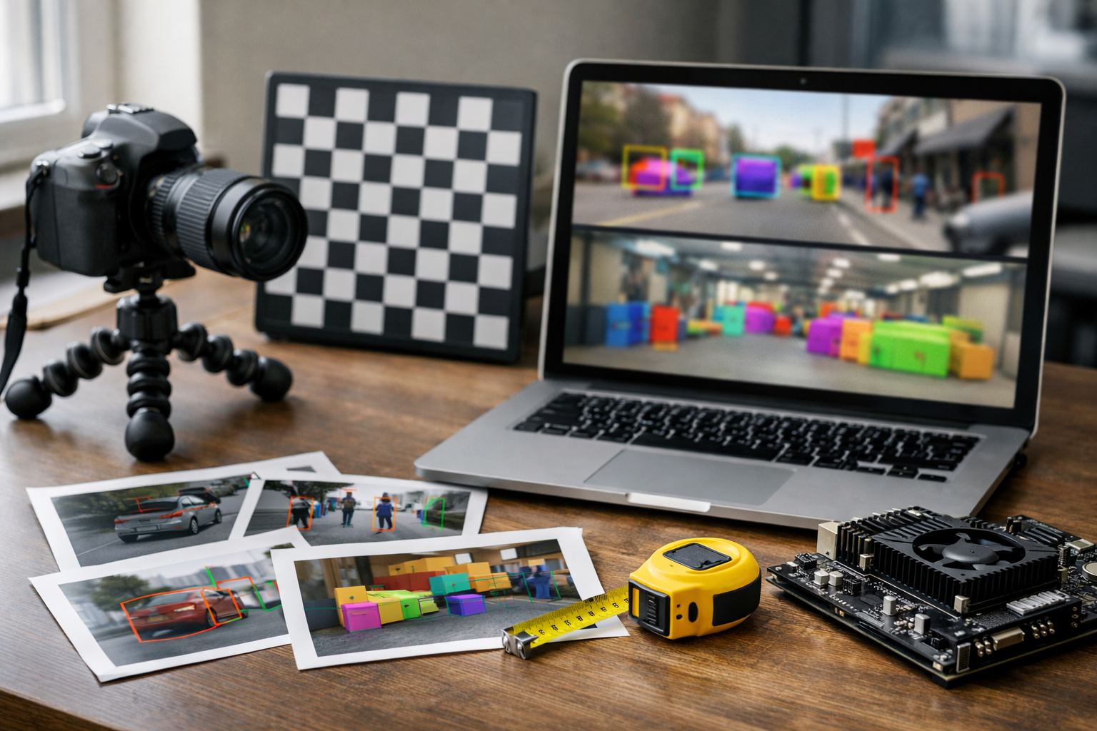
The mini-lab outcome in this chapter is a QA-ready export package. For each validation image, export: (1) the predicted mask as a PNG (palette or grayscale IDs), (2) an overlay visualization (image + semi-transparent mask, plus boundaries), and (3) a small JSON summary (per-class pixel counts, instance counts, confidence stats). Overlay audits catch alignment bugs instantly: a one-pixel shift from preprocessing, a flipped axis from RLE decoding, or a class-ID mapping error. They also reveal qualitative failures like jagged edges, holes, and merged objects that metrics may underemphasize.

• Overlay checklist: verify colors map to correct classes; boundaries line up with visible edges; ignored regions are not penalized; and instance colors are unique per object.
• Common pitfall: evaluating on post-processed masks but exporting raw masks (or vice versa), causing QA reviewers to see different results than the metric report.

Finish by storing artifacts with traceability: model checkpoint ID, dataset version, and preprocessing config. In real teams—and in certification-style grading—being able to reproduce a mask from a run is as important as the mask’s score.

Most production MOT systems are tracking-by-detection: you run a detector per frame and then link detections into trajectories. This formulation is modular and certification-friendly because you can test each component (detector quality, association quality, motion assumptions) independently. It also aligns with real-world constraints: you may swap detectors (YOLO/RT-DETR/Faster R-CNN) without rewriting the tracker, and you can version each stage for reproducible experiments.

End-to-end MOT models (jointly predicting tracks across time) exist, but they often require more specialized training data, more compute, and tighter coupling between model and dataset. They can be strong in benchmarks, yet harder to debug when a track fails—did the network miss the object, confuse identities, or mis-handle occlusion? In a certification workflow, tracking-by-detection is typically the baseline, and end-to-end approaches are considered only after you can clearly articulate your baseline’s failure modes.

Create track-ready data early. Frame sampling matters: labeling every frame may be wasteful for slow motion, but sparse sampling can break association learning and make evaluation misleading. Use a sampling policy tied to object speed and camera FPS (e.g., label every frame for fast interactions; every 2–3 frames for slow scenes, then interpolate only if your labeling tool supports it with review). IDs must be consistent across the entire clip; define rules for when an identity is “the same” (e.g., same physical car even if partially occluded) and when to start a new ID (e.g., object leaves the scene and re-enters much later without reliable re-identification cues). Explicit occlusion labeling (occluded/fully visible/truncated) becomes valuable later for diagnosing why association breaks.

• Common mistake: mixing annotation conventions across labelers (some restart IDs after occlusion, others keep them). This inflates ID switches and makes metrics uninterpretable.
• Practical outcome: you can describe your tracking task precisely (short-term MOT vs long-term re-ID) and ensure the dataset matches that task.

Motion modeling provides a “physics prior” that stabilizes tracking under detector noise and short occlusions. The standard baseline is a Kalman filter with a constant-velocity model, usually tracking a bounding box state such as center (x, y), scale/area, aspect ratio, and their velocities. In practice, you do not need a perfect motion model; you need a model that is stable, easy to tune, and predictable when it fails.

A constant-velocity Kalman filter assumes the object continues moving with similar velocity between frames. This works well for pedestrians and vehicles in typical FPS ranges, but it can struggle with abrupt turns, camera cuts, or strong perspective effects. Your engineering judgment appears in choosing process noise (how much you “trust” the model vs measurements). If process noise is too low, tracks lag behind sudden motion and association fails. If it is too high, the prediction becomes loose and increases incorrect matches.

Gating is the key practical concept: you restrict candidate matches to those that are plausible given the predicted state. Common gating strategies use Mahalanobis distance from the Kalman prediction, or simpler geometric gates such as maximum center distance or minimum IoU with the predicted box. Gating improves speed (fewer candidates for Hungarian matching) and reduces catastrophic ID switches by preventing absurd associations across the frame.

• Tip: tune gating thresholds on a validation video set that includes crowded scenes and mild occlusion. A gate that works in sparse scenes may fail in crowds.
• Common mistake: ignoring camera motion. If the camera pans, constant velocity in image coordinates may be invalid; consider compensating with global motion (Section 4.6) or increasing process noise.

As a baseline MOT implementation, combine detector outputs with a motion filter: predict all tracks, gate candidate detections, then associate. This “detector + motion” system is the minimal engine you must get working before adding appearance features.

Data association answers: which detection belongs to which existing track in the current frame? The standard solution is to build a cost matrix between predicted tracks and detections, then solve a bipartite assignment with the Hungarian algorithm. The design work lies in defining the cost and thresholds so that the algorithm behaves sensibly when detections are missing, duplicated, or noisy.

A simple baseline cost is IoU distance (e.g., cost = 1 − IoU between predicted box and detected box). IoU works when boxes overlap reliably, but it can fail during fast motion or partial occlusion where overlap is small. To mitigate this, gating (Section 4.2) ensures you only compare plausible candidates, and you can incorporate a motion distance term such as normalized center distance.

To reduce ID switches in crowded scenes, add an appearance cost from an embedding network (e.g., a lightweight ReID model that outputs a feature vector per detection). In practice, you compute cosine distance between track appearance (a running average or a gallery of recent embeddings) and detection embedding, then blend it with IoU cost: total_cost = w_iou * iou_cost + w_app * app_cost. Tuning is not optional. You must choose (1) the weights, (2) the acceptance threshold (max cost allowed), and (3) how embeddings are updated over time (aggressive updates can “drift” the identity when the tracker is wrong).

• Engineering judgment: if your detector is strong but objects look similar (uniforms, identical products), appearance should carry more weight. If lighting changes rapidly, appearance may be unstable and motion/geometry should dominate.
• Common mistake: using appearance embeddings without normalizing features or without validating distance distributions; thresholds then become arbitrary and brittle.

In a certification-ready workflow, log association decisions per frame: the chosen match, IoU, appearance distance, and whether gating excluded alternatives. These logs make later ID switch analysis evidence-based rather than guesswork.

Occlusion is the main reason simple trackers fail. When an object is partially hidden, the detector may output a shifted box; when fully hidden, it may output nothing. Track management is your policy layer: how long to keep a track alive without detections, how to handle re-entry, and how to prevent identity “stealing” when two objects cross.

Start with clear lifecycle states: tentative (new track not yet trusted), confirmed (stable track), and lost (temporarily unmatched). A common rule is “confirm after N consecutive matches” and “delete after T missed frames.” N and T depend on FPS and scene dynamics. High FPS scenes can tolerate small T; low FPS or intermittent detection requires larger T to prevent fragmentation.

For short-term occlusion, motion prediction bridges the gap: keep the track in a lost state and try to match it again when detections return. For longer-term occlusion or when objects leave and re-enter, you need re-identification logic. This is where appearance embeddings are most valuable: maintain a small gallery of recent embeddings per track and match returning detections based on appearance similarity plus coarse location constraints.

Occlusion labeling in your dataset becomes a practical tool here. By marking frames as “occluded,” you can stratify evaluation: do ID switches cluster around heavy occlusion? Are deletions happening too early during occlusion segments? You can then tune T, adjust gating, or reduce detector confidence thresholds during occlusions if your detector tends to drop objects when partially visible.

• Common mistake: letting a lost track keep updating its appearance embedding when the match confidence is low. This causes identity drift and makes later re-ID worse.
• Practical outcome: you can explain and justify your track birth/death rules, and you can make them consistent with your labeling conventions (especially whether IDs persist through long disappearances).

Tracking metrics can be intimidating because they combine detection quality and identity consistency. For certification and real engineering work, focus on what each metric punishes so you can connect failures to fixes.

MOTA (Multi-Object Tracking Accuracy) aggregates false positives, false negatives, and ID switches into a single score. It is useful as a headline metric, but it can hide why a system is failing. For example, improving detector recall can increase false positives and unexpectedly reduce MOTA even if trajectories “look” better. Treat MOTA as an outcome, not a guide.

IDF1 focuses on identity preservation: it measures how well predicted track identities align with ground truth over time. If users care about “same person across the scene,” IDF1 is often closer to perceived quality than MOTA. ID switches, track fragmentation, and incorrect re-linking after occlusion will hurt IDF1 even when detection is strong.

HOTA (Higher Order Tracking Accuracy) was designed to balance detection and association quality more explicitly than MOTA. It provides insight into the trade-off: you can have good detection but poor association, or vice versa. In practice, HOTA is helpful for comparing trackers that make different engineering choices (strong gating vs strong appearance, aggressive track deletion vs long persistence).

• Workflow: report MOTA + IDF1 + HOTA on the same validation set, then break down errors by scenario (crowd density, occlusion level, camera motion).
• Common mistake: optimizing only one metric and declaring victory. A tracker that “games” MOTA by deleting tracks early can look good numerically but be unusable for analytics that require persistent IDs.

When you analyze ID switches, do not stop at the count. Identify where they occur (crossing paths, occlusion, re-entry) and connect each cluster to a concrete knob: association threshold, appearance weight, gating size, or track lifecycle parameters.

Debugging tracking is fundamentally visual. Your primary artifact should be an annotated tracking video: bounding boxes with track IDs, color-coded states (tentative/confirmed/lost), and optional overlays of predicted vs detected boxes. This is the mini-lab deliverable: generate review videos that allow you (or an evaluator) to audit track behavior frame by frame.

Three recurring failure modes deserve structured diagnosis. Drift happens when a track slowly slides off the object, often due to detector bias under occlusion or an overly confident motion model. Fixes include increasing process noise, tightening gating to avoid weak matches, or using detector box refinement (e.g., rerun detection in a cropped region around predictions). Fragmentation occurs when one ground-truth object becomes multiple short tracks. It often indicates track deletion too early (T too small), detector confidence threshold too high, or gating too strict. ID switches appear when two tracks swap identities, commonly during close interactions or crossings; strengthen appearance cost, add a “no-match” threshold to avoid forced assignments, and consider two-stage association (first high-confidence IoU matches, then appearance-based recovery).

Camera motion is a special case because it breaks naive assumptions about image-space velocity. If the camera pans or zooms, many objects share a global motion vector. A practical remedy is global motion compensation: estimate frame-to-frame transformation (e.g., homography from background features) and warp predictions before association. Even a rough compensation can reduce false mismatches in handheld or moving-platform footage.

• Mini-lab checklist: (1) sample frames and label IDs consistently, including occlusion flags; (2) run baseline detector+Kalman tracker; (3) add appearance embeddings and tune thresholds; (4) compute MOTA/IDF1/HOTA; (5) render a review video highlighting drift, fragmentation, and ID switches.
• Common mistake: changing multiple thresholds at once. Trackers are sensitive; adjust one variable, rerun, and save artifacts so improvements are attributable.

The practical outcome of debugging is not only higher metrics—it is confidence. A certification-ready tracker is one where you can explain why it fails in specific scenes, what you changed to address it, and how you verified the fix with metrics and visual evidence.

Domain shift is the umbrella term for “the world changed.” To respond correctly, you must name the type of change, because each one suggests different fixes and different evaluation slices.

Covariate shift means the input distribution changes while the underlying task remains the same. Examples: blur from motion, low-light noise at night, new camera sensor, rain/snow, or stronger compression artifacts from a bandwidth limiter. Your labels are still “correct,” but the pixels look different. The most effective first response is data-centric: collect a small, targeted set under the new conditions, and run stress tests with corruption transforms (Gaussian blur, defocus blur, JPEG/H.264 artifacts, gamma shifts, fog/rain overlays) to measure sensitivity.

Label shift means the frequency of classes changes. A warehouse model trained when forklifts were common may face mostly pallet jacks after an operational change. Accuracy can appear to drop simply because the prior distribution changed, and fixed thresholds become suboptimal. Countermeasure: re-check per-class precision/recall and recalibrate thresholds or sampling/weighting. Importantly, do not “fix” label shift by inventing augmentation; fix it by aligning your evaluation and training sampling to the new class mix.

Concept drift means the mapping from input to label changes—often due to changed definitions. If “defect” is redefined (new tolerance), or a tracking ID policy changes (what counts as a new identity), then old labels no longer represent the current task. The remedy is governance: update labeling guidelines, retrain with consistent ground truth, and version your label schema. Common mistake: silently mixing old and new label policies, which produces irreducible confusion in training and meaningless metrics.

For certification-ready workflow, create a “shift matrix” document: list expected conditions (day/night, rain, blur levels, bitrate tiers), which shift type they represent, and what data/metrics you will use to detect degradation. This sets you up to mitigate shift with intent instead of reacting randomly after failures.

Augmentation is not decoration; it is a hypothesis about what variations matter. The key is to mimic your deployment pipeline. If your camera stream is H.264 at variable bitrate, then JPEG-only augmentation may miss the artifact patterns that actually break your model. If you deploy on rolling-shutter mobile cameras, motion blur and wobble matter more than photometric jitter.

Do: build a corruption suite that matches the stress-test list: blur (motion/defocus), low-light (gamma + Poisson noise), weather (fog/rain overlays), and compression (JPEG + video compression approximations). Use severity levels and record performance curves: accuracy vs. blur sigma, mAP vs. bitrate tier, Dice vs. illumination level. This gives engineering judgement: you can say “we remain above 0.5 mAP until JPEG quality 30, then degrade sharply.”

Do: combine geometric and photometric transforms cautiously for detection/segmentation. For segmentation, heavy elastic deformations can create unrealistic boundaries and teach the model artifacts. For tracking, augmentations that reorder frames or break temporal consistency can harm motion/appearance learning; prefer per-sequence consistent photometric transforms rather than random per-frame jitter.

Don’t: over-augment until the model underfits clean data. A common mistake is applying maximal blur/noise to every sample. Instead, use a mixture schedule: most samples lightly augmented, a smaller fraction heavily corrupted. Another mistake is adding synthetic weather overlays that do not match the optics (e.g., rain streaks at the wrong scale), which can reduce real-world robustness because the model learns “synthetic cues.”

Synthetic data can fill gaps, but you must validate it like a dataset: check annotation correctness, class balance, and whether textures/lighting are plausible. A practical rule: synthetic data is best for expanding geometry (viewpoints, rare poses, occlusion patterns), while real data is essential for sensor noise and compression quirks. Always report metrics on a real, held-out “shifted” set; never claim robustness based only on synthetic evaluation.

Production failures often come from misinterpreting confidence scores. A detector’s “0.9” is not automatically a 90% probability of correctness, especially under shift. Calibration is the practice of aligning confidence with empirical correctness so that thresholds mean something.

Start by plotting reliability diagrams on your validation set and on corrupted/shifted slices. If you can, use temperature scaling (for classification heads) or class-wise calibration for detection scores. For segmentation, consider calibrating per-pixel probabilities (or at least calibrating an aggregate mask confidence such as mean logit over the predicted region). For tracking, calibration shows up as gating: how strict you are when associating detections to tracks, and how you handle low-confidence detections to reduce ID switches.

Next, define thresholds as policies, not magic numbers. Use two thresholds when appropriate: a high threshold for “act” (e.g., trigger an event), and a lower threshold for “observe” (e.g., show a box but do not trigger). For instance segmentation, you may require both box confidence and mask quality (IoU proxy) before a downstream robot action. For tracking, you may require consistent evidence over N frames before declaring an object “present.” These policies reduce flicker and false alarms caused by compression bursts or sudden exposure shifts.

• Abstention: when confidence is low or inputs are out-of-distribution, return “unknown” and log the sample for review.
• Fallback behaviors: degrade gracefully: switch to a simpler detector at lower resolution, pause automation and request human review, or rely more on motion model when appearance is unreliable (e.g., low light) while limiting track lifetime to avoid drift.

Common mistake: optimizing mAP and then setting a single threshold that looks good on average. In real systems, the cost of false positives vs. false negatives is asymmetric. Tie thresholds to risk: document which errors are unacceptable, then validate on the stress-test suite. Your deployment artifact should include: chosen thresholds per class, expected precision/recall on key slices (night, rain, compressed), and the abstention/fallback trigger conditions.

Robustness includes meeting latency and throughput requirements consistently. A model that is accurate but misses real-time constraints will fail downstream (stale tracks, delayed alarms, poor UX). Start with a latency budget: break end-to-end time into capture/decode, pre-processing, inference, post-processing (NMS, mask rendering), tracking association, and output/serialization.

Define your targets explicitly: FPS (average), frame latency (p50), and tail latency (p95/p99). Tail latency matters because jitter causes dropped frames and unstable tracking. Next, match these targets to hardware constraints: CPU-only edge device, GPU workstation, or embedded accelerator. The same architecture behaves differently depending on memory bandwidth and kernel support.

Key engineering levers:

• Resolution: the largest driver of compute. For small objects, downscaling harms recall; validate a few candidate resolutions and pick the lowest that meets recall on your smallest critical objects.
• Batching: improves throughput on GPUs but increases latency. For live video, micro-batching (e.g., batch=2–4) may be acceptable if it stays within p95 constraints; for offline analytics, larger batches maximize throughput.
• Pipeline parallelism: overlap decode/preprocess with inference; use pinned memory and asynchronous transfers where applicable.
• Post-processing cost: NMS and mask upsampling can dominate at high object counts. Profile them; sometimes limiting max detections or using class-agnostic NMS reduces latency spikes.

Common mistake: reporting only model FPS from a benchmark script that excludes decoding and post-processing. Your certification-ready deliverable is a latency budget sheet with measured timings on target hardware, including realistic input formats (compressed streams, not raw frames) and worst-case scenes (many objects, heavy weather artifacts). This ensures your tracking metrics (MOTA/HOTA) are not silently undermined by dropped frames or delayed associations.

Quantization and pruning are practical tools to meet performance budgets, but they can introduce accuracy cliffs—especially under the same edge cases you are trying to handle. Approach them as controlled experiments with explicit acceptance criteria.

Quantization reduces precision (e.g., FP32 to INT8) to speed inference and reduce memory. Two common paths are post-training quantization (PTQ) and quantization-aware training (QAT). PTQ is faster to implement but is more sensitive to activation outliers; QAT usually preserves accuracy better but requires training time and careful setup. For detectors/segmenters, small-object recall and boundary quality (Dice/IoU near edges) are often the first to degrade. For tracking, degraded appearance embeddings can increase ID switches even if detection mAP looks similar.

Pruning removes weights or channels. Structured pruning (channels/blocks) is more deployment-friendly than unstructured sparsity unless your hardware supports sparse acceleration. A practical approach is: prune conservatively, fine-tune briefly, then re-evaluate on both clean and corrupted slices.

Validation rule: do not validate compression only on the clean validation set. Re-run your robustness suite: blur, low light, weather, and compression tiers, plus any domain-shifted holdout you maintain. Record deltas in mAP/IoU/Dice and tracking metrics (MOTA/HOTA, IDF1, ID switches). Often, INT8 may keep mAP within 1 point but increase ID switches substantially because association becomes less stable under low light. If tracking is a requirement, that is a deployment blocker.

Common mistake: calibrating INT8 with random images rather than representative samples. Your calibration set should include typical lighting, typical compression, and some edge conditions. If you deploy multiple cameras, include a mix; otherwise, quantization may “lock in” bias toward one sensor’s statistics.

Once deployed, you need evidence that the system is still operating within its validated envelope. Monitoring is not just uptime; it is model health and data health. Design monitoring hooks during development so you can answer, “What changed?” when performance degrades.

Data quality monitoring checks whether inputs resemble what the model expects: brightness histograms, blur scores (e.g., Laplacian variance), compression/bitrate indicators, frame drops, and camera tampering signals. Track these per camera and over time. Sudden shifts (e.g., blur score spike) often explain metric changes without any model issue.

Metric drift monitoring requires proxies because ground truth is scarce in production. Useful proxies include: average detection confidence, class distribution of predictions, fraction of frames with zero detections, track lifetimes, ID switch rate proxies (e.g., frequent track fragmentation), and segmentation mask area distributions. When you do have periodic labels (audits), compute official metrics (mAP, IoU/Dice, MOTA/HOTA) on a rotating, stratified sample that includes known edge conditions.

Alert design should avoid noise. Use multi-signal alerts (e.g., confidence drop + blur increase) and rate limits. Define “actionable thresholds” tied to impact: an alert that triggers a ticket, a rollback, or a human review workflow. Also log “abstention events” from Section 5.3; abstention spikes are often the earliest sign of covariate shift.

• Common mistake: monitoring only average confidence. Confidence can remain high while being wrong under concept drift.
• Common mistake: ignoring tail latency. If p99 latency spikes, tracking quality can degrade even if per-frame detection is fine.

End this chapter by implementing two artifacts: (1) a robustness test suite you can run locally and in CI (clean + corruption severities + shifted slices), and (2) a latency budget sheet with measured timings and FPS targets. Then wire monitoring hooks to log the exact features your test suite perturbs (blur, brightness, compression), closing the loop between validation and real-world operation.

The fastest way to fail a capstone is to pick a scenario that is ambiguous, unmeasurable, or too large. Start by choosing a scenario with clear objects and predictable camera dynamics. Good examples: “warehouse pallet tracking from a fixed CCTV,” “players and ball in a single broadcast angle,” or “road users from a dashcam.” Your scenario choice should determine the task mix: detection for coarse localization, segmentation when pixel-accurate boundaries matter, and tracking to maintain identities across frames.

Write requirements as testable statements. Instead of “track well,” define thresholds tied to metrics: e.g., “HOTA ≥ 55 on the held-out test set,” “MOTA ≥ 70 with ID switches < 1 per 200 frames,” “mask mAP@0.5:0.95 ≥ 0.35,” or “Dice ≥ 0.80 for a semantic class.” Include latency and hardware constraints if deployment is part of your story (e.g., “≥ 15 FPS on CPU-only laptop” or “real-time on T4 GPU”).

• Risks: occlusion, motion blur, class imbalance, annotation ambiguity, domain shift (day/night), and camera jitter.
• Scope controls: limit classes (2–5), define “ignore regions,” restrict to one viewpoint, and declare what you won’t solve (e.g., “no re-identification across scene cuts”).
• Success metrics: pick one primary metric per task (mAP for detection, Dice/IoU for segmentation, HOTA or MOTA for tracking) plus 1–2 secondary metrics for diagnosis.

Common mistake: setting a single metric goal without specifying the evaluation protocol. Your requirements must include the dataset split strategy, the IoU thresholds, confidence thresholds policy, and whether you use class-agnostic vs class-aware evaluation. This is the “capstone spec” an examiner expects: concise, measurable, and aligned with your scenario.

Design the system as modules connected by data contracts. This makes debugging possible and allows you to swap models without rewriting everything. A practical high-level flow is: Frame loader → Detector → (optional) Segmenter → Tracker → Renderer/Exporter. Each module should have a clear input/output schema (e.g., numpy arrays, tensors, or JSON lines) and a versioned definition of fields.

Your unified dataset is deliverable #1. Unify detection boxes, segmentation masks, and tracking IDs in one canonical format, even if some tasks are missing for certain samples. Many teams use COCO-style for detection/segmentation and MOT-style for tracking, but the key is consistency. Define image/frame identifiers, category IDs, bounding boxes (xywh vs xyxy), masks (RLE/polygons), and track IDs per frame. Include “ignore” flags for ambiguous regions and a policy for crowd instances.

• Labeling guide: specify class definitions, occlusion rules, truncation rules, minimum size, and when to mark “ignore.” Include 5–10 visual examples of edge cases.
• Evaluation scripts: provide a single command to compute detection mAP, segmentation IoU/Dice, and tracking HOTA/MOTA on the same split; lock metric library versions.
• Data contracts: define coordinate systems, image resizing/letterboxing rules, and how transforms are reversed at inference for correct metrics.

Common mistake: mixing preprocessing between training and inference (e.g., letterbox during training but center-crop during demo), which produces “mystery” metric drops. Treat preprocessing as part of the contract: same resize policy, same normalization, and explicit mapping back to original coordinates. For tracking, be explicit about which representation is fed to the tracker (raw detector boxes, refined mask boxes, or mask centroids) and how confidence gating is applied.

Deliverable #2 is not merely “trained models,” but reproducible training runs: configs, seeds, checkpoints, and logs that can be replayed. Create a single source of truth for hyperparameters (YAML/JSON) and load it everywhere—training, evaluation, and export. Record model architecture, input resolution, augmentation policy, optimizer settings, class mapping, and dataset commit hash.

Reproducibility has three layers. First, set seeds (Python, NumPy, framework seed) and deterministic flags where feasible, understanding that some GPU ops remain nondeterministic. Second, capture the environment: framework versions, CUDA/cuDNN versions, and key dependencies. Third, persist artifacts: best checkpoint, last checkpoint, training curves, confusion matrices, qualitative visualizations, and the exact evaluation outputs used in your report.

• Experiment tracking: use a tool (or a structured folder layout) to store run metadata and artifacts; name runs by scenario + date + key change.
• Ablation discipline: change one factor at a time (anchor sizes, loss weights, augmentation strength, tracker association thresholds).
• Checkpoint criteria: pick the best checkpoint based on a validation metric aligned with your primary goal (e.g., HOTA on a validation video subset, not just detector mAP).

Common mistake: optimizing detection alone and assuming tracking will improve automatically. In practice, tracking stability depends on detection recall, localization jitter, and confidence calibration. Trackers suffer when box sizes fluctuate frame-to-frame; a modest improvement in temporal consistency can reduce ID switches more than a small mAP gain. Consider post-processing (e.g., box smoothing) only if it is included consistently in evaluation and disclosed in your report.

Deliverable #3 is an integrated inference pipeline that a reviewer can run with one command and that outputs a demo video. Package your project with a simple CLI: input can be a video file, a folder of frames, or a camera device; output should include a rendered video (overlays for boxes/masks/IDs), plus machine-readable results (JSON/CSV) for further evaluation.

Export is part of certification readiness because it forces you to confront deployment constraints: dynamic shapes, unsupported ops, and post-processing differences. Provide at least one export path (ONNX or TorchScript) and verify it numerically against the native model on a fixed set of inputs. If you use ONNX Runtime or TensorRT, document expected speedups and limitations.

• CLI design: flags for model paths, confidence thresholds, IoU/NMS settings, tracker parameters, device selection, and output directory.
• Versioning: version your dataset schema, model weights, and inference code together; tag releases (e.g., v1.0-capstone) and store a changelog.
• Deterministic demo: keep a small “demo clip” in the repo (or provide a download script) so results are reproducible for reviewers.

Common mistake: a demo video that looks good but cannot be regenerated. Examiners value repeatability: a single command that reconstructs the exact overlays and metrics. Another common pitfall is mismatched post-processing between training evaluation and packaged inference (NMS differences, mask thresholding differences). Your package should include the same post-processing used to compute reported metrics, or explicitly label the demo as “illustrative” and keep metrics tied to the evaluation script.

Your report is where you demonstrate judgment, not just numbers. Start with the capstone spec: scenario, dataset size, split strategy, and success metrics. Then present results in a narrative that explains tradeoffs and failure modes. Use robust metrics: mAP for detection, IoU/Dice for segmentation, and MOTA/HOTA for tracking. Include not only final scores but also diagnostic slices: performance by object size, lighting condition, motion intensity, and occlusion level.

A strong report connects ablations to outcomes. For detection, you might compare anchor-based vs anchor-free or different input resolutions; for segmentation, compare loss functions (Dice vs BCE+Dice) or boundary refinement; for tracking, compare association metrics (IoU-only vs motion+appearance), and show how ID switches change. Keep ablations small and honest: 3–6 focused experiments that each answer a question.

• Visual evidence: include side-by-side frames showing correct vs failed cases, with annotations for why the system failed (missed detection, mask leakage, identity swap).
• Failure taxonomy: categorize issues into data (label noise, missing classes), model (underfit/overfit), and pipeline (preprocessing mismatch, thresholding).
• Metric integrity: declare thresholds, IoU settings, and whether you tuned parameters on validation only.

Common mistake: presenting metrics without context or claiming causality without evidence. If your tracking improves after changing detector confidence threshold, explain the mechanism: fewer false positives reduce track fragmentation, but too high a threshold increases missed detections and hurts HOTA. Make that tradeoff explicit. Finally, include the exact commands used to compute each metric and link them to saved artifacts (predictions files, logs, checkpoint hashes).

The mock exam portion of the capstone is about speed and reliability under constraints. Practice timed troubleshooting drills that mirror real incidents: a sudden metric drop after a refactor, an ONNX export mismatch, a tracker that explodes with ID switches on one clip, or segmentation masks that shift due to resizing. The goal is not to memorize answers, but to follow a repeatable diagnostic sequence: reproduce, isolate, measure, and fix.

Use a final readiness checklist that maps directly to certification outcomes. Your portfolio should allow an evaluator to (1) understand the scenario and requirements in one page, (2) reproduce training or at least run evaluation on provided checkpoints, and (3) run the end-to-end demo pipeline. Keep the presentation professional: clean repository structure, clear READMEs, and pinned versions.

• Checklist: dataset schema documented; labeling guide with edge cases; evaluation scripts run from scratch; configs and seeds saved; checkpoints and logs available; export verified; CLI demo works; report includes failure analysis.
• Troubleshooting habits: always compare preprocessing; validate coordinate transforms; inspect a few raw predictions; check class mappings; confirm metric library settings.
• Portfolio packaging: include “quickstart” commands, expected outputs, and a small reproducible demo clip.

Common mistake: focusing only on model training and leaving integration until the end. Integration work (data contracts, exports, CLI, versioning) often surfaces hidden assumptions that affect metrics. Treat packaging and reporting as first-class engineering tasks. If your capstone runs reliably, produces defensible metrics, and explains its own weaknesses, you are ready for both the certification and a real CV role.