Computer Vision — Beginner
Build a beginner-friendly app that finds faces and sorts photos for you.
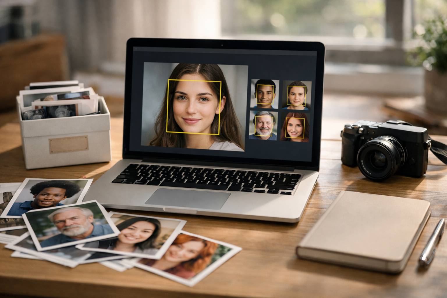
This beginner-friendly course is designed like a short, practical technical book: you’ll start with zero knowledge and finish with a working “Smart Photo Album Organizer” that can scan a folder of photos, find faces, mark key facial landmarks (like eyes and mouth), and sort photos into simple groups. You don’t need to know AI, math, or coding ahead of time—we build every idea from the ground up using plain language and small steps.
By the end, you’ll have a small program you can run on your computer that:
Face detection answers: “Where are the faces in this image?” Landmark detection adds: “Where are the important points on the face?” Together, they let you crop faces consistently, handle multiple people in the same photo, and create outputs that are easy to review. This course focuses on using reliable pre-trained models so you can build something useful without needing to train anything from scratch.
You’ll begin with the basics: what an image is (pixels and color channels), how to run a Python script, and how to open and save photos. Then you’ll add face detection, followed by landmark detection, and learn how to turn your results into clean files you can reuse (like CSV metadata and face thumbnails). Finally, you’ll learn a simple method for grouping similar faces so your photos can be organized into person-like collections.
Each chapter ends with a checkpoint so you always know what “done” looks like. If something breaks, you’ll have saved outputs (proof images and logs) to help you see what happened and fix it.
This course avoids heavy theory and focuses on clear mental models:
Because faces are sensitive data, you’ll also learn basic safety habits: getting consent, avoiding risky uses, storing outputs securely, and keeping your project local. The goal is to help you build something helpful (like personal photo organization) while understanding the responsibility that comes with face technology.
If you want a gentle, hands-on introduction to face and landmark detection that results in a real project you can run and share, this course is for you. Register free to begin, or browse all courses to compare learning paths.
Computer Vision Engineer and Beginner Curriculum Designer
Sofia Chen builds practical computer vision features for consumer apps, with a focus on face analysis and photo workflows. She designs beginner-first lessons that turn complex topics into small, confidence-building steps.
This course builds a beginner-friendly “Smart Photo Album Organizer”: you point it at a folder of photos, it scans each image, finds faces, marks key facial landmarks (eyes, nose, mouth), saves annotated copies, and writes a CSV report you can sort or filter. Later chapters add the “smart” part: grouping photos into simple albums using face similarity basics. In this first chapter, your goal is more fundamental and more important: a calm, reliable setup where you can process one photo end-to-end with a short Python script.
Computer vision projects can feel intimidating because they mix software setup, file handling, and visual debugging. We will reduce fear by using a consistent workflow: (1) read an image from disk, (2) verify what you loaded, (3) apply one operation, (4) save the result, (5) repeat on a folder. Each step has a clear output you can check. If something breaks, you’ll know which step failed and why.
By the end of this chapter you will have: a project folder with a predictable structure; a working Python environment; a script that opens, displays (optionally), and saves an image; and the engineering habit of verifying inputs/outputs before moving on. That checkpoint makes the next steps—face detection and landmark visualization—feel straightforward instead of mysterious.
outputs/ folder.In the sections below, we’ll build the mental model (what images are in code), choose tools, install them safely, and write your first reliable script. Keep one principle in mind: computer vision is not magic—it is disciplined data processing with images as the data.
Practice note for What this course builds: the Smart Photo Album Organizer: document your objective, define a measurable success check, and run a small experiment before scaling. Capture what changed, why it changed, and what you would test next. This discipline improves reliability and makes your learning transferable to future projects.
Practice note for Install Python the easy way and verify it works: document your objective, define a measurable success check, and run a small experiment before scaling. Capture what changed, why it changed, and what you would test next. This discipline improves reliability and makes your learning transferable to future projects.
Practice note for Set up a project folder and run your first script: document your objective, define a measurable success check, and run a small experiment before scaling. Capture what changed, why it changed, and what you would test next. This discipline improves reliability and makes your learning transferable to future projects.
Practice note for Open, display, and save an image successfully: document your objective, define a measurable success check, and run a small experiment before scaling. Capture what changed, why it changed, and what you would test next. This discipline improves reliability and makes your learning transferable to future projects.
Practice note for Checkpoint: you can process one photo end-to-end: document your objective, define a measurable success check, and run a small experiment before scaling. Capture what changed, why it changed, and what you would test next. This discipline improves reliability and makes your learning transferable to future projects.
Practice note for What this course builds: the Smart Photo Album Organizer: document your objective, define a measurable success check, and run a small experiment before scaling. Capture what changed, why it changed, and what you would test next. This discipline improves reliability and makes your learning transferable to future projects.
Practice note for Install Python the easy way and verify it works: document your objective, define a measurable success check, and run a small experiment before scaling. Capture what changed, why it changed, and what you would test next. This discipline improves reliability and makes your learning transferable to future projects.
Practice note for Set up a project folder and run your first script: document your objective, define a measurable success check, and run a small experiment before scaling. Capture what changed, why it changed, and what you would test next. This discipline improves reliability and makes your learning transferable to future projects.
Computer vision is the practice of teaching a computer to answer questions about images. In everyday terms: you give the computer a photo, and it gives you structured information back—“there is a face here,” “these are the eye positions,” or “these two photos likely contain the same person.” The computer does not “see” like humans do; it performs measurements on pixel values and uses models (algorithms trained on many examples) to map those measurements to useful outputs.
In this course, the outputs you’ll care about are visual and easy to verify. A face detector returns rectangles (bounding boxes) around faces. A landmark detector returns points (or small groups of points) for facial features like eyes, nose, and mouth. When you draw those results back onto the image, you get immediate feedback: if the box is offset or landmarks are wrong, you can see it.
It’s helpful to think of the Smart Photo Album as a small pipeline rather than a single “AI step.” The pipeline starts with files on disk, loads them into memory, converts them into the formats your tools expect, runs detection, then writes results back to disk (annotated images + a CSV file). Most beginner frustration comes from skipping verification—e.g., running a detector on an image that failed to load, or using the wrong color channel order.
Today’s checkpoint is intentionally simple: if you can reliably load and save a photo with a small change (like drawing a line or resizing), you have proven your environment, dependencies, and file paths. That eliminates most setup fear before we add face detection logic.
An image on your computer is a grid of pixels. Each pixel stores numbers that represent color and brightness. In most photos, each pixel has three color channels: red, green, and blue. When you load an image in Python, you typically get a 3D array shaped like (height, width, channels). If an image is 800×600, you might see something like (600, 800, 3). That is not trivia—many bugs become obvious once you check the shape.
One detail matters a lot for beginners: different libraries use different channel orders. Many image tools and tutorials talk in RGB order (red, green, blue). OpenCV, however, loads images by default in BGR order (blue, green, red). This is not a deep concept, but it is a frequent source of “my colors look weird” issues. If you display an OpenCV image with a library that expects RGB (like Matplotlib), blues and reds may swap.
cv2.cvtColor(img, cv2.COLOR_BGR2RGB) before plotting with Matplotlib.You will also encounter grayscale images, where the array shape is (height, width) with a single channel. Some detectors work on grayscale for speed; others expect color. The engineering judgement here is to always read the documentation for the specific function you call—and then confirm the actual array you pass matches that expectation.
Finally, remember that most pixel values are integers in the range 0–255 (8-bit). When you later compute face embeddings for similarity, you may normalize values or convert to floating point—but for this chapter, your goal is simply to load the image correctly and preserve it when saving.
We will use three pieces of tooling throughout the course. First is Python, because it’s readable, widely supported, and has excellent computer vision libraries. Second is OpenCV (cv2), which handles the practical tasks: reading/writing images, drawing boxes and points, resizing, color conversion, and running classic detectors when needed. Third is a facial landmark library that provides pre-trained models to locate eyes, nose, and mouth reliably.
You will see multiple landmark options in the ecosystem. Two common beginner-friendly choices are MediaPipe Face Mesh and dlib’s landmark predictor (or wrappers around it). The exact library choice can depend on your operating system and how easily you can install dependencies. The course workflow stays the same whichever you use: pass an image in, receive landmarks out, then visualize them with OpenCV drawing utilities.
For engineering judgement, prioritize tools that: (1) install cleanly on your machine, (2) have stable APIs, and (3) produce outputs you can validate visually. A slightly less “fancy” model that runs everywhere is better than a perfect model you cannot install. Early on, reliability beats sophistication.
In this chapter you will not yet implement face detection and landmarks fully, but you will set up the environment so that adding those calls later is a small incremental change. Think of this as laying a clean foundation: once imports and file IO work, model steps become just another function call in the pipeline.
“No fear setup” means two things: you install Python and libraries in a way that does not break other projects, and you troubleshoot systematically rather than randomly. The safest path for beginners is to use a dedicated virtual environment per project. This keeps dependencies isolated so that upgrading OpenCV for this course won’t silently break a different script you wrote last month.
Recommended approach: install a modern Python (3.10+ is usually a good target), then create a virtual environment inside your project folder. On Windows, the Python installer has a checkbox to “Add Python to PATH”—enable it. On macOS, installing via python.org or a package manager is fine; the key is that python (or python3) runs from your terminal.
python --version (or python3 --version).python -m venv .venv.venv\Scripts\activate; macOS/Linux: source .venv/bin/activatepip install opencv-python (and later, the landmark library chosen by the course).When something fails, avoid guessing. Use a checklist: (1) Are you in the right environment? (2) Are you installing with the environment’s pip? (3) Does python -c "import cv2; print(cv2.__version__)" work? A common mistake is installing packages globally while running scripts in a different interpreter.
Troubleshooting also means knowing when not to fight your system. If a landmark library requires compilation and you hit compiler errors, consider switching to an alternative that provides prebuilt wheels for your OS. Your goal is to learn computer vision workflows, not spend a weekend debugging build tools. Make the pragmatic choice that keeps you moving.
Most beginner bugs in computer vision are not “AI bugs”—they are file path and IO bugs. Your script must locate an image file, load it, confirm it loaded, then write an output file somewhere you can find. OpenCV’s cv2.imread returns None if the path is wrong or the file can’t be read. If you forget to check for None, the next line will crash with a confusing error about shapes or types.
A reliable pattern is: build absolute paths from a known project root, avoid manual string concatenation, and always check results. In Python, pathlib.Path makes this clean and cross-platform (Windows vs macOS/Linux path separators).
img = cv2.imread(str(image_path))if img is None: raise FileNotFoundError(...)cv2.imwrite(str(output_path), img_out)Displaying images is optional and depends on your environment. In a desktop Python run, cv2.imshow can work, but it requires a GUI and a cv2.waitKey call. In notebooks, Matplotlib is often easier. The key engineering judgement: don’t treat display as your only verification method. Saving an output image is more reliable because it works in headless environments and creates a persistent artifact you can inspect later.
For your first script, do something visibly obvious: draw a rectangle in the corner or write text on the image using cv2.putText. Then save it as outputs/test_annotated.jpg. If that file appears and looks correct, you have proven: your environment is correct, OpenCV is installed, paths are correct, and you can write results—exactly what you need before you add face boxes and landmarks.
Organization is a technical skill in computer vision because you will generate many intermediate artifacts: annotated images, CSV files, and debug outputs. A clean project structure prevents you from overwriting results or losing track of which run produced which output. It also makes batch processing (scanning a whole folder) simpler because inputs and outputs are clearly separated.
Use a predictable layout from day one. Here is a practical structure that matches the Smart Photo Album workflow:
smart_album/ (project root)inputs/ (your original photos; do not modify)outputs/ (annotated images, reports)src/ (Python code)src/main.py (entry point you run)requirements.txt (pinned dependencies)Even in Chapter 1, adopt the habit of never editing files in inputs/. Always write to outputs/. This mirrors how you will later batch-scan folders: the script loops over inputs/, processes each photo, and writes a corresponding annotated image plus a row in a CSV file. That separation also supports “reruns”: you can delete outputs/ and regenerate everything without risking your originals.
For your first run, keep the interface simple: hardcode a single file name like inputs/photo1.jpg. Once that works, you can extend to command-line arguments (e.g., --input, --output) or a folder scan. The engineering judgement is incrementalism: confirm one photo end-to-end before multiplying complexity across 500 photos.
Checkpoint (end of chapter): you can run python src/main.py and it reads one image from inputs/, makes a visible modification, and writes a new image into outputs/. If you can do that consistently, you are ready to add face bounding boxes and landmark points in the next chapter without fighting your setup.
1. What is the main goal of Chapter 1 before starting face detection and landmarks?
2. Which workflow best matches the chapter’s recommended approach to reduce fear and debug issues?
3. Why does the chapter emphasize verifying inputs and outputs at each step?
4. What practical outcome should you be able to demonstrate by the end of Chapter 1?
5. Which statement best reflects the chapter’s mental model of computer vision work?
In Chapter 1 you set up the project idea: a “smart photo album” that can scan a folder of images and later help you group them. The first technical step is not “Who is this person?”—it is simply “Is there a face here, and where is it?” That task is called face detection. Detection is the gatekeeper for everything else: if you can’t find the face reliably, you can’t crop it, align it, extract landmarks, or compare it to other faces.
This chapter is intentionally practical. You’ll build a minimal workflow: load an image, run a pre-trained detector locally, handle one face, handle many faces, handle no faces, and draw a bounding box back onto the image so you can visually verify results. You’ll also learn what the detector’s “confidence score” means, how to tune a couple of settings to reduce false positives or missed faces, and how to save “proof images” to debug batch runs. By the end, you should be able to run detection over a small folder of photos and feel confident that your face boxes are correct most of the time.
One engineering judgement to adopt early: always validate with visuals. Face detection can look “done” if you only print counts to the console, but it can be wildly wrong (boxes on posters, boxes on background faces you don’t care about, or boxes that cut off chins). The fastest way to build intuition is to draw boxes on images and inspect a sample set. We’ll make that a habit in this chapter.
We will also set expectations: face detection is not magic. It does not understand identity, emotion, or intent; it only estimates whether a region looks like a face based on patterns learned from large datasets. That means quality depends on lighting, pose, blur, and resolution. The goal for beginners is not perfection—it’s a robust baseline that you can iterate on.
Keep your focus narrow: in this chapter, success means “face boxes work on a small photo set.” Landmarks and grouping come next, but you’ll already be laying the groundwork by producing clean crops and trustworthy detections.
Practice note for What “face detection” means and what it does not do: document your objective, define a measurable success check, and run a small experiment before scaling. Capture what changed, why it changed, and what you would test next. This discipline improves reliability and makes your learning transferable to future projects.
Practice note for Detect a single face and draw a box: document your objective, define a measurable success check, and run a small experiment before scaling. Capture what changed, why it changed, and what you would test next. This discipline improves reliability and makes your learning transferable to future projects.
Practice note for Detect multiple faces and handle “no face found”: document your objective, define a measurable success check, and run a small experiment before scaling. Capture what changed, why it changed, and what you would test next. This discipline improves reliability and makes your learning transferable to future projects.
Practice note for Tune detection settings for better results: document your objective, define a measurable success check, and run a small experiment before scaling. Capture what changed, why it changed, and what you would test next. This discipline improves reliability and makes your learning transferable to future projects.
Practice note for Checkpoint: face boxes work on a small photo set: document your objective, define a measurable success check, and run a small experiment before scaling. Capture what changed, why it changed, and what you would test next. This discipline improves reliability and makes your learning transferable to future projects.
Computer vision terms are often mixed up, and that confusion causes wrong design choices. Let’s separate three tasks you will see throughout this course: detection, recognition/verification, and identification. They sound similar, but they answer different questions and produce different outputs.
Face detection answers: “Where are the faces?” The input is an image; the output is one or more bounding boxes (rectangles) and usually a confidence score for each box. Detection does not tell you who the person is. In your smart album, detection is used to locate faces so you can crop, align, and store them for later steps.
Face recognition (often called verification) answers: “Is this the same person as that?” The input is typically two face crops; the output is a similarity score (or yes/no). This is the basis for grouping photos by person. Recognition assumes you already have good face crops—so it depends on detection quality.
Face identification answers: “Who is this person from a known set?” The input is a face crop and a database of labeled people; the output is the best-matching identity (or “unknown”). Identification requires a gallery of known people and has higher privacy and product implications than detection.
A practical workflow mindset: detection is a geometry and localization problem, recognition is an similarity problem, and identification is a label assignment problem. When debugging, keep these layers separate. If recognition is failing, first confirm detection boxes are correct and not cutting off key parts of the face. Many beginners try to “fix recognition” when the real issue is that detection is inconsistent.
In this chapter you will treat the detector as a tool that produces candidates. Your job is to decide how strict to be (via thresholds), how to handle edge cases (no faces, many faces), and how to record evidence (proof images) so you can improve settings systematically rather than guessing.
You do not need to know every detail of modern deep learning to use a face detector effectively, but you do need a mental model of what it’s doing. The simplest model is: the detector looks at many regions of the image and asks, “Does this region look like a face?” It repeats that at different positions and sizes, then returns the best regions.
Historically this was literally implemented as a sliding window that scanned across the image at multiple scales. Many modern detectors (CNN-based) are faster and more elegant, but the behavior is similar: they evaluate many candidate boxes (sometimes called anchors) across a grid, score them, and then clean up the results.
Two key operations happen after scoring:
This model explains common observations. If you see two boxes on the same face, NMS may be too permissive or you may be combining results from multiple scales. If you miss a face far in the background, the face may be too small relative to the detector’s minimum size or the image was downscaled too aggressively before detection.
It also suggests practical tuning levers. Detectors often provide options like min_face_size (ignore very small faces), scale_factor (how aggressively to build the image pyramid), and a confidence threshold. Changing these affects speed and recall. For a smart album, you typically want a balanced setup: detect clear faces reliably while avoiding spending lots of time chasing tiny faces in the distance.
Finally, remember that the detector is not “understanding a face” the way humans do. It is matching learned patterns. That’s why it can be fooled by face-like shapes, and why strong lighting changes (backlit windows, harsh shadows) can reduce confidence even when the face is obvious to you.
For a beginner-friendly, local setup, a strong choice is OpenCV’s pre-trained DNN face detector (ResNet-SSD). It runs on CPU, works offline, and returns bounding boxes plus confidence. The goal here is to write a small script that loads an image, runs detection, and prints the results. Keep it minimal first; you can refactor into functions once it works.
First, install dependencies:
pip install opencv-python
Then download the model files (once) into a folder like models/:
deploy.prototxtres10_300x300_ssd_iter_140000_fp16.caffemodelNow run detection on a single photo:
import cv2

img = cv2.imread("photos/sample.jpg")
if img is None:
    raise ValueError("Could not read image")

h, w = img.shape[:2]
net = cv2.dnn.readNetFromCaffe(
    "models/deploy.prototxt",
    "models/res10_300x300_ssd_iter_140000_fp16.caffemodel",
)

blob = cv2.dnn.blobFromImage(
    img, 1.0, (300, 300), (104.0, 177.0, 123.0), swapRB=False, crop=False
)
net.setInput(blob)
detections = net.forward()  # shape: [1, 1, N, 7]

for i in range(detections.shape[2]):
    conf = float(detections[0, 0, i, 2])
    x1 = int(detections[0, 0, i, 3] * w)
    y1 = int(detections[0, 0, i, 4] * h)
    x2 = int(detections[0, 0, i, 5] * w)
    y2 = int(detections[0, 0, i, 6] * h)
    print(i, conf, (x1, y1, x2, y2))
Important engineering details beginners miss:
img is None so batch runs don’t silently skip broken files.At this stage you may see multiple detections including low-confidence ones. That’s normal. In the next section you’ll filter by confidence and draw the boxes so you can judge whether the detector is behaving correctly.
Printing coordinates is not enough—draw boxes. Visualization turns face detection from “numbers” into something you can evaluate in seconds. You’ll also handle three practical cases: a single face, multiple faces, and no face found.
Start by filtering detections with a confidence threshold, then draw rectangles and labels:
import os
import cv2

CONF_TH = 0.6
img = cv2.imread("photos/sample.jpg")
h, w = img.shape[:2]

# ... (load net, forward pass) ...

faces = []
for i in range(detections.shape[2]):
    conf = float(detections[0, 0, i, 2])
    if conf < CONF_TH:
        continue
    x1 = max(0, int(detections[0, 0, i, 3] * w))
    y1 = max(0, int(detections[0, 0, i, 4] * h))
    x2 = min(w - 1, int(detections[0, 0, i, 5] * w))
    y2 = min(h - 1, int(detections[0, 0, i, 6] * h))
    faces.append((conf, x1, y1, x2, y2))

# Sort best-first (useful when you “expect one main face”)
faces.sort(key=lambda t: t[0], reverse=True)

out = img.copy()
for conf, x1, y1, x2, y2 in faces:
    cv2.rectangle(out, (x1, y1), (x2, y2), (0, 255, 0), 2)
    label = f"face {conf:.2f}"
    cv2.putText(out, label, (x1, max(0, y1 - 8)),
                cv2.FONT_HERSHEY_SIMPLEX, 0.6, (0, 255, 0), 2)

if len(faces) == 0:
    cv2.putText(out, "NO FACE FOUND", (20, 40),
                cv2.FONT_HERSHEY_SIMPLEX, 1.0, (0, 0, 255), 2)

os.makedirs("outputs", exist_ok=True)
cv2.imwrite("outputs/sample_boxed.jpg", out)
Notice the small but critical choices:
Tuning settings is mostly about trade-offs. If you set CONF_TH too high, you’ll miss faces in dim light or at an angle. Too low, and you may get boxes on background objects or portraits on posters. For a first checkpoint, try 0.5–0.7 and adjust after reviewing proof images from a small set of photos (10–30 images). Your aim is consistent boxes, not perfect recall.
When a detector fails, it often fails in predictable ways. Knowing these patterns helps you debug calmly and choose sensible mitigations instead of randomly changing code. In a smart album, you will see all of these in real family photos.
Lighting issues are the biggest source of missed detections. Backlighting (bright window behind a person) can turn the face into a dark silhouette, reducing detector confidence. Harsh overhead lighting creates shadows under eyes and noses that distort the normal face pattern. Practical mitigation: don’t jump immediately to “better model.” First try lowering the confidence threshold slightly, and consider running detection on the original resolution rather than a downscaled thumbnail. If you control image ingestion, avoid re-encoding aggressively.
Angle and pose matter because many detectors are strongest on near-frontal faces. Profiles, faces tilted down, or extreme wide-angle selfies can reduce confidence or shift the box. Practical mitigation: test your detector on your target photo style. If your album includes lots of side profiles (sports photos, candid shots), you may need a more robust model later. For now, be aware that your “no face found” cases may not be bugs; they may be limitations.
Occlusion includes sunglasses, masks, hands covering the face, hair across eyes, or a baby held against someone’s shoulder. Detectors typically need enough visible structure (eyes/nose/mouth region) to fire. Practical mitigation: lower threshold carefully, but watch false positives. Also consider a rule like “ignore very small boxes” so you don’t accept random clutter as faces when trying to recover occluded faces.
Small faces and motion blur show up in group photos, concerts, and action shots. A face that is only 20–30 pixels tall may be below the detector’s practical limit. Blur removes the sharp edges that detectors rely on. Practical mitigation: process at higher resolution, avoid downscaling before detection, and accept that some distant faces won’t be detected reliably without a specialized model.
False positives commonly happen on posters, paintings, faces on T-shirts, mannequin heads, or even round objects with face-like patterns. This matters for albums because you don’t want a “person” cluster made from background art. Practical mitigation: increase the confidence threshold, require a minimum face size, and later (in grouping) require consistency across multiple photos before creating a new album identity.
Batch processing is where face detection becomes real engineering. When you scan hundreds of photos, some will fail for reasons you didn’t anticipate. If you don’t save evidence, you will be stuck with vague logs like “0 faces found,” and you won’t know whether the issue is your threshold, image reading, orientation, or model limitations.
A simple best practice is to always save a “proof image” for each input: the original photo with boxes (or a clear “NO FACE FOUND” stamp). Store them in a separate folder so you can review them quickly and compare before/after changes to thresholds.
Here is a minimal folder-scanning script pattern:
import os
import glob
import cv2

in_dir = "photos"
out_dir = "outputs/proof"
os.makedirs(out_dir, exist_ok=True)

paths = sorted(glob.glob(os.path.join(in_dir, "*.jpg")))
for path in paths:
    img = cv2.imread(path)
    if img is None:
        continue

    # run detector -> faces list
    # draw boxes onto `out`

    base = os.path.splitext(os.path.basename(path))[0]
    cv2.imwrite(os.path.join(out_dir, f"{base}_proof.jpg"), out)
Engineering judgement: do not save only “failures.” Save everything during early development. Seeing correct outputs alongside incorrect ones teaches you what “good” looks like and prevents you from overfitting to weird cases. Once stable, you can switch to saving only failures or only a sample.
Also, preserve traceability. Use filenames that let you map a proof image back to the original input easily. If you later produce a CSV (in a later chapter) with columns like filename, face_index, confidence, and box coordinates, you’ll be able to reproduce any result.
Checkpoint for this chapter: pick a small photo set (10–30 images) that represents your real data (indoor, outdoor, group shots). Run your batch script, open the proof folder, and visually confirm that bounding boxes are mostly correct, that multiple faces are detected in group photos, and that “no face found” appears only when you agree there is no usable face. If not, adjust your confidence threshold and rerun until you have a baseline you trust.
1. What is the main goal of face detection in the smart photo album workflow described in Chapter 2?
2. Why does the chapter call face detection a “gatekeeper” for later steps like cropping, landmarks, and comparing faces?
3. When running detection over a folder of photos, what practice does the chapter recommend to quickly validate whether detection is actually working?
4. Which handling is part of the minimal practical workflow emphasized in Chapter 2?
5. What is the purpose of tuning detection settings (including interpreting confidence scores) as described in the chapter?
Face detection tells you where a face is; landmark detection tells you what parts of that face are where. In a smart photo album, landmarks are the bridge between a rough rectangle and a consistent, usable crop of a face—no matter if the head is tilted, the photo is rotated, or the person is slightly off-center. This chapter focuses on the most common “beginner set” of landmarks: eyes, nose, and mouth points (often a few points per feature).
Why this matters practically: if you batch-scan hundreds of photos, face boxes alone produce thumbnails that feel random—sometimes the forehead is cut off, sometimes the chin, and sometimes the face is diagonal. Landmarks let you normalize those thumbnails. They also help you match each detected face to the correct set of feature points when multiple faces appear in one image, a frequent real-world scenario in family albums and group shots.
We’ll move from concepts to a repeatable workflow: detect faces, estimate landmarks for each face, visualize points to verify quality, then align and crop a consistent face thumbnail you can reuse in later chapters (e.g., face similarity grouping). Along the way you’ll see common mistakes (wrong coordinate assumptions, mixing faces, and drawing overlays on the wrong image copy) and the engineering judgment behind robust choices.
The rest of the chapter is organized into six sections: what landmarks represent, which models you can use out of the box, how coordinates work, how to visualize for debugging, the face-alignment idea, and finally a practical function you can call in a batch script.
Practice note for What landmarks are and why they matter: document your objective, define a measurable success check, and run a small experiment before scaling. Capture what changed, why it changed, and what you would test next. This discipline improves reliability and makes your learning transferable to future projects.
Practice note for Find landmarks on one face and draw them: document your objective, define a measurable success check, and run a small experiment before scaling. Capture what changed, why it changed, and what you would test next. This discipline improves reliability and makes your learning transferable to future projects.
Practice note for Handle multiple faces and match landmarks to the right box: document your objective, define a measurable success check, and run a small experiment before scaling. Capture what changed, why it changed, and what you would test next. This discipline improves reliability and makes your learning transferable to future projects.
Practice note for Use landmarks to align/crop a consistent face thumbnail: document your objective, define a measurable success check, and run a small experiment before scaling. Capture what changed, why it changed, and what you would test next. This discipline improves reliability and makes your learning transferable to future projects.
Practice note for Checkpoint: clean face thumbnails saved for later steps: document your objective, define a measurable success check, and run a small experiment before scaling. Capture what changed, why it changed, and what you would test next. This discipline improves reliability and makes your learning transferable to future projects.
Practice note for What landmarks are and why they matter: document your objective, define a measurable success check, and run a small experiment before scaling. Capture what changed, why it changed, and what you would test next. This discipline improves reliability and makes your learning transferable to future projects.
Practice note for Find landmarks on one face and draw them: document your objective, define a measurable success check, and run a small experiment before scaling. Capture what changed, why it changed, and what you would test next. This discipline improves reliability and makes your learning transferable to future projects.
Practice note for Handle multiple faces and match landmarks to the right box: document your objective, define a measurable success check, and run a small experiment before scaling. Capture what changed, why it changed, and what you would test next. This discipline improves reliability and makes your learning transferable to future projects.
Facial landmarks are named points placed on specific facial structures—corners of the eyes, tip of the nose, corners of the mouth, the outline of the lips, and sometimes eyebrows and jawline. Think of them as a “map” of the face. A face bounding box is one rectangle; landmarks are many coordinates that describe the face’s geometry. Even with just a few landmarks (left eye center, right eye center, nose tip, left mouth corner, right mouth corner), you can infer head tilt, estimate where the face is actually centered, and create a crop that is consistent from photo to photo.
Landmarks matter because faces are not rigid objects. People turn their heads, cameras are held at angles, and expressions change. A detector that outputs only a rectangle cannot tell whether the face is rotated within that rectangle. Landmarks reveal that rotation: the line between the eyes is a strong cue for roll (tilt), and the relative position of nose-to-mouth helps confirm that the points are sensible (sanity check). In engineering terms, landmarks add structure that you can exploit for alignment, normalization, and quality control.
A common mistake is expecting landmarks to be perfect “anatomy points” in every photo. In reality, they are model predictions. Glasses, occlusions, motion blur, extreme angles, or very small faces can shift points. Your goal is not perfection; your goal is consistent enough landmarks to drive a stable crop and to detect obvious failures early (for example, eyes swapped or mouth points outside the face box).
You rarely train a landmark model from scratch for a beginner project. The standard approach is to use a pre-trained model that outputs landmarks given an image (and sometimes a face region). Two popular options are:
Model choice is an engineering trade-off. If your goal is a smart album with reliable thumbnails, a smaller landmark set is often enough and easier to reason about. A 5-point predictor (or extracting a subset from a larger mesh) provides exactly what we need: stable eye and mouth anchors. Larger meshes shine when you need detailed facial geometry, but they also increase the risk of overfitting your pipeline to points you don’t actually need.
Another practical judgment: decide whether your landmark model expects a face box as input. Many pipelines run face detection first, then run landmark estimation inside each box. This is usually faster and reduces false landmarks on background patterns. If your landmark tool does its own face detection internally, be careful when multiple faces are present—you’ll need a consistent mapping between the face boxes you draw and the landmark sets you compute.
Common mistakes include mixing color channel conventions (OpenCV loads BGR, some models expect RGB) and forgetting to handle image resizing. If you resize an image for speed, you must scale landmark coordinates back to the original size before drawing or cropping. Build that scaling into your code early so it doesn’t become a hidden bug when you switch from a single test image to a folder of photos.
Landmarks are coordinates, and coordinate misunderstandings are the #1 cause of “my points are in the wrong place.” In typical image processing, a pixel coordinate is written as (x, y) where x increases to the right and y increases downward. However, NumPy arrays index images as img[y, x] (row first, then column). You must be consistent about when you are using (x, y) tuples versus array indexing.
Landmark libraries may output coordinates in different formats:
x_px = x_norm * width and y_px = y_norm * height.When handling multiple faces, store coordinates in a structured way. A practical pattern is: for each detected face box, keep a dictionary with bbox and landmarks. If landmarks are computed on a crop, immediately convert them into full-image coordinates and store both. This reduces “which coordinate space is this?” confusion later when you visualize or align.
Two sanity checks help catch errors early: (1) landmark points should lie inside or near the face bounding box; (2) the left eye’s x-coordinate should be less than the right eye’s x-coordinate in a normal (non-mirrored) image. If either check fails consistently, it usually indicates a coordinate conversion mistake (normalized vs pixels, ROI offsets, or swapped width/height).
Visualization is not just “nice to have”—it’s your fastest debugging tool. Before you trust landmarks for cropping and alignment, draw them. The simplest overlay is a small filled circle at each landmark point. Use distinct colors for different facial features so you can see at a glance if the model is confused (for example, mouth points placed near an eye because the face was too small).
A practical workflow for one face is:
cv2.rectangle.cv2.circle.When there are multiple faces, visualization helps you verify you’re matching the right landmarks to the right box. One robust strategy is to compute landmarks per face ROI: crop by each detected box, run landmark estimation, then shift points back into full-image coordinates. Then draw using a per-face color or label. If your library returns multiple landmark sets from the full image, match each set to the nearest face box by comparing the landmark centroid (average x/y) to each box center.
Common mistakes: drawing on a resized copy but saving the original; forgetting to convert RGB/BGR, which can make you think detection failed when it’s really color-space; and silently rounding too early. Keep landmark points as floats during computation, and only convert to ints at the final drawing step.
The practical outcome of this section is a reliable “debug render” image you can generate for any photo. Later, when you batch-scan a folder, you’ll be grateful you can quickly spot patterns of failure (tiny faces, side profiles, heavy blur) and decide how to handle them (skip, fallback crop, or different thresholds).
Face alignment means transforming a face so key features land in consistent locations—typically making the eyes level (removing roll) and scaling the face so the distance between the eyes is constant. This is how professional pipelines create uniform thumbnails. Alignment is not about beautification; it’s about consistency so later steps (like face similarity embeddings) get cleaner inputs.
The simplest alignment uses the two eye landmarks. Compute the angle of the line from left eye to right eye:
dx = x_right - x_left, dy = y_right - y_leftangle = atan2(dy, dx) (in radians; convert to degrees for OpenCV)Then rotate the image around a chosen center (often the midpoint between eyes or the face box center) using cv2.getRotationMatrix2D and cv2.warpAffine. After rotation, the eyes become horizontal. Next, decide a target scale (e.g., set inter-eye distance to a fixed number of pixels) and apply scaling as part of the same affine transform or by resizing the cropped region.
Engineering judgment: alignment can be overdone. For very small faces or uncertain landmarks, rotating aggressively can worsen quality. A practical rule is to clamp extreme angles (e.g., ignore alignment if |angle| > 45° unless you specifically want to handle rotated photos) and require a minimum face size before aligning. Also, remember that some photos are mirrored (selfie cameras). If your pipeline later relies on “left” and “right” semantics, treat the eyes simply as two points and compute a stable angle regardless of which is which.
Alignment sets you up for consistent cropping: once faces are upright, you can crop with predictable margins above the eyes and below the mouth. That predictability is what makes a smart album feel polished.
At this point, you have all building blocks; now you turn them into a function you can call for one image or a whole folder. The goal is a repeatable function that takes an image and a face detection result and returns a clean thumbnail plus metadata you can store (box, landmarks, alignment angle, output path). Treat this like a small API you will reuse later.
A practical function signature looks like:
extract_face_thumbnail(image, bbox, landmarks, out_size=(160,160), margin=0.35)Inside, implement a consistent sequence:
out_size with cv2.resize and a good interpolation (area for downscale).Handling multiple faces becomes straightforward if you loop over detected boxes, compute landmarks per box, and call the same function for each face index. Always store outputs in a structured folder (e.g., thumbnails/) and keep a CSV row per extracted face with: image filename, face index, bbox coordinates, landmark coordinates (or a simplified subset), alignment angle, and thumbnail path. This checkpoint—clean thumbnails saved for later steps—is your “contract” with the rest of the course. If thumbnails are consistent here, face similarity grouping later will be easier and more accurate.
Common mistakes in productionizing this: forgetting that rotations change image extents (some pixels rotate out of frame), mixing coordinate spaces after rotation, and not handling failures gracefully. Your function should never crash the batch; it should either skip a face with a logged reason or produce a fallback thumbnail. In real photo libraries, you will encounter edge cases constantly, and robustness is a feature.
1. In a smart photo album pipeline, what problem do landmarks solve that face bounding boxes alone do not?
2. When an image contains multiple faces, why are landmarks especially useful beyond visualization?
3. Which workflow best reflects the repeatable process described for producing usable face thumbnails?
4. Which outcome most directly reflects the chapter’s stated goal for later steps like face similarity grouping?
5. Which is an example of an engineering mistake the chapter warns about that can break landmark drawing or cropping logic?
In the previous chapters, you learned how to detect faces and (optionally) landmarks on a single image. That’s useful for experimenting, but a “smart photo album” becomes real when it can process an entire folder—hundreds or thousands of photos—reliably and repeatably. This chapter is about turning a messy pile of files into clean, structured data you can search, sort, and build albums from later.
When engineers say “turn photos into data,” they mean: (1) scan a folder, (2) run the same pipeline on every valid image, (3) save the outputs in a predictable place, and (4) write down what happened in a machine-readable format. The most beginner-friendly format is a CSV file: one row per detected face (or per image), containing file name, face coordinates, and any metadata you care about (e.g., blur score).
Good batch processing is less about clever algorithms and more about discipline: handling weird filenames, skipping broken images, making sure each output can be traced back to its input, and recording failures so you can fix them later. You’ll also add “quality checks” so the pipeline doesn’t waste time saving tiny faces or faces from nearly black frames. Finally, you’ll generate a contact sheet (a grid image) of detected face crops so you can visually audit results without opening files one by one.
As you build this chapter’s script, keep a simple goal in mind: make your pipeline boring. “Boring” means the same inputs always produce the same outputs, and failures are captured as data instead of crashing your run.
Practice note for Scan a folder of images safely and quickly: document your objective, define a measurable success check, and run a small experiment before scaling. Capture what changed, why it changed, and what you would test next. This discipline improves reliability and makes your learning transferable to future projects.
Practice note for Write results to a CSV (faces found, coordinates, file names): document your objective, define a measurable success check, and run a small experiment before scaling. Capture what changed, why it changed, and what you would test next. This discipline improves reliability and makes your learning transferable to future projects.
Practice note for Generate a contact sheet of detected faces: document your objective, define a measurable success check, and run a small experiment before scaling. Capture what changed, why it changed, and what you would test next. This discipline improves reliability and makes your learning transferable to future projects.
Practice note for Add simple quality checks (too small, too blurry, too dark): document your objective, define a measurable success check, and run a small experiment before scaling. Capture what changed, why it changed, and what you would test next. This discipline improves reliability and makes your learning transferable to future projects.
Practice note for Checkpoint: one command creates outputs for a whole folder: document your objective, define a measurable success check, and run a small experiment before scaling. Capture what changed, why it changed, and what you would test next. This discipline improves reliability and makes your learning transferable to future projects.
Practice note for Scan a folder of images safely and quickly: document your objective, define a measurable success check, and run a small experiment before scaling. Capture what changed, why it changed, and what you would test next. This discipline improves reliability and makes your learning transferable to future projects.
Practice note for Write results to a CSV (faces found, coordinates, file names): document your objective, define a measurable success check, and run a small experiment before scaling. Capture what changed, why it changed, and what you would test next. This discipline improves reliability and makes your learning transferable to future projects.
Practice note for Generate a contact sheet of detected faces: document your objective, define a measurable success check, and run a small experiment before scaling. Capture what changed, why it changed, and what you would test next. This discipline improves reliability and makes your learning transferable to future projects.
Batch processing starts with one idea: your face detector should not care whether it’s seeing photo #1 or photo #10,000. The loop is the “factory line,” and every step inside it must be predictable: load → detect → save → record. A common beginner mistake is writing code that works for one image but silently reuses state (like an old filename or an old detection result) on the next iteration. Keep everything inside the loop explicit.
In Python, you typically start by collecting file paths with pathlib.Path. Use rglob if you want subfolders; use iterdir for a single folder. Sort the paths to make runs deterministic (useful for debugging and for comparing outputs between versions).
from pathlib import Path

input_dir = Path("photos")
paths = sorted([p for p in input_dir.rglob("*") if p.is_file()])

for path in paths:
    # 1) load image
    # 2) run face detection + landmarks
    # 3) save annotated image / face crops
    # 4) append rows to CSV data structure
    pass
Build your loop so it never “forgets” where it is. Print occasional progress (e.g., every 50 images) and keep counts: images scanned, images loaded, faces found, images skipped. Those counters become your first sanity check: if you scanned 800 files but only loaded 30, you probably filtered extensions incorrectly; if you loaded 800 but found zero faces, your detector settings are wrong or images were resized too aggressively.
To generate a contact sheet later, you can collect face crops (as small arrays) during the loop, but be mindful of memory. For a beginner-friendly version, collect only a limited number (e.g., the first 200 crops) or save crops to disk and build the contact sheet from files after the run.
Real photo folders are messy. You’ll see .jpg, .jpeg, .png, sometimes .webp, and occasionally non-images disguised with image-like names. Clean file handling means: (1) choose what you support, (2) detect and skip unsupported files, and (3) never crash the whole batch because one file is corrupted.
Start with a small allowlist of extensions, compared case-insensitively. It’s tempting to accept everything, but beginners get better results by being strict first and adding formats later.
ALLOWED = {".jpg", ".jpeg", ".png"}

ext = path.suffix.lower()
if ext not in ALLOWED:
    # record skip reason and continue
    continue
Next, wrap image loading in try/except. If you’re using OpenCV, cv2.imread returns None on failure; if you’re using PIL, it may raise an exception. Either way, treat “can’t load” as a data point. Record a row in a separate “images” CSV (or a log list) with a status like load_failed. Avoid print-only error handling—printed errors are hard to audit later.
Also decide on skipping rules. Examples: skip images below a minimum size (e.g., width < 200 px), skip images with alpha channels if your pipeline can’t handle them, or skip if the file path contains temporary folders. The key judgement is to skip intentionally and consistently, not randomly. Every skip should have a reason you can count.
Common mistake: assuming every path is unique and stable. If you process subfolders, different photos can share the same filename (e.g., IMG_0001.jpg). You must base output naming on relative paths or a hash, not only the basename. This will matter when you start saving crops and annotated images.
A CSV is your “memory” of the batch run. Images are heavy and human-friendly; CSV is lightweight and machine-friendly. Later chapters will use this CSV to group photos into albums, search for faces, and compare similarity. A good rule is: store one row per detected face, not one row per image, because a single photo can contain multiple people.
At minimum, each face row should include: input file path (relative), face index, bounding box (x, y, w, h), and a detection confidence if your detector provides it. If you also compute landmarks, store them as separate columns (e.g., left_eye_x, left_eye_y, etc.) or as a JSON-like string column for flexibility. Beginners often try to store Python lists directly; instead, serialize consistently.
import csv

fieldnames = [
  "image_relpath", "face_id",
  "x", "y", "w", "h",
  "conf",
  "left_eye_x", "left_eye_y",
  "right_eye_x", "right_eye_y",
  "nose_x", "nose_y",
  "mouth_x", "mouth_y",
  "blur", "brightness", "too_small", "too_dark", "too_blurry"
]

with open("outputs/detections.csv", "w", newline="", encoding="utf-8") as f:
    writer = csv.DictWriter(f, fieldnames=fieldnames)
    writer.writeheader()
    # writer.writerow(...) for each detected face
Include both raw numbers and simple flags. The raw numbers (blur score, brightness) let you adjust thresholds later without reprocessing. The flags (too_dark) make it easy to filter quickly. Engineering judgement: prefer storing more context now, because re-running a long batch just to add one column is frustrating.
Another common mistake is mixing coordinate systems. If you resize images for speed, your detections may be in resized coordinates. Always record what coordinate space you are saving. A practical approach: save detections in the coordinate system of the image you used for detection, and also store the resize scale factor so you can map back to the original if needed.
Once you start saving outputs—annotated images, face crops, contact sheets—you need a naming scheme that prevents collisions and makes it obvious where a file came from. An audit trail means you can answer: “Which input produced this crop?” and “Which settings produced this CSV?” without guessing.
Use a single outputs/ folder with clear subfolders, for example:
outputs/annotated/ — original photo with boxes/landmarks drawnoutputs/faces/ — cropped facesoutputs/reports/ — CSV files and run metadataoutputs/contact_sheet.jpg — grid previewFor each face crop, include enough information in the filename to make it unique and traceable: relative image path (sanitized), face index, and maybe bounding box. Example: vacation_2023_day1_IMG_0042__face02_x120_y80_w90_h90.jpg. If that feels too long, use a stable hash of the relative path and store the original path in the CSV.
Also save a small run manifest (a simple text or JSON file) containing: timestamp, input folder, allowed extensions, resize policy, quality thresholds, and versions of key libraries. Beginners skip this, then later can’t reproduce why results changed after “minor edits.” Reproducibility is part of correctness.
Finally, build the contact sheet as a visual audit. A contact sheet should not be “pretty”; it should be diagnostic. Use consistent crop sizes (e.g., 128×128), arrange in a grid, and optionally label each tile with the source image ID and face index. If you see many blank tiles, misaligned crops, or tiny faces, you know to revisit thresholds and resizing.
Not every detected face is worth keeping. In a smart album, low-quality detections create noise: tiny faces from crowd shots, blurry frames from motion, or dark images where landmarks are unreliable. You can reduce this noise with simple, explainable rules. The goal is not to be perfect; it’s to make the dataset cleaner so later steps (like face similarity grouping) behave better.
Too small: if the face bounding box is below a threshold (e.g., width or height < 40 px in the detection image), mark it too_small=1. Tiny faces often lead to poor landmark placement and unstable embeddings later. You can still keep them, but label them so you can filter.
Too blurry: a classic beginner metric is the variance of the Laplacian (OpenCV). Low variance suggests low detail. Choose a threshold by sampling: compute the blur score for 30 faces you consider “ok” and 30 you consider “bad,” then pick a cut that separates them reasonably.
Too dark: compute mean brightness on the face crop (convert to grayscale and take the average). If the mean is below a threshold (e.g., < 50 on 0–255), flag it. Darkness can come from underexposure or backlighting; either way, it often reduces detector confidence.
Common mistake: setting thresholds before looking at your own data. Camera sources vary wildly. Use the contact sheet to calibrate thresholds. Engineering judgement here is iterative: run on a small subset, adjust, then run the full folder.
Batch scanning can be slow if you run detection on full-resolution photos from modern phones (3000–6000 px wide). Most face detectors don’t need that much detail for initial localization. Resizing is the easiest performance win, but it introduces a key responsibility: keep coordinates consistent and don’t resize so aggressively that you miss faces.
A practical strategy is to resize so the longer side is capped, for example at 1280 px. Compute a scale factor, resize once, run detection on the resized image, and record the scale factor in your CSV. If you later need coordinates in the original image, multiply by 1/scale. Keep this mapping explicit; otherwise you will draw boxes in the wrong place or crop the wrong region.
# pseudo-logic
max_side = 1280
scale = min(1.0, max_side / max(h, w))
resized = resize(image, fx=scale, fy=scale)
# detect on resized
# store scale in CSV
Resizing affects quality checks too. “Too small” should be evaluated in the detection coordinate space (resized image), because that matches what the detector saw. But if you save crops from the original image, you may want a second “too small in original pixels” check to avoid saving postage-stamp faces.
To reach the chapter checkpoint—one command creates outputs for a whole folder—keep performance predictable: avoid loading images twice, don’t keep huge arrays in memory, and save incrementally. Write CSV rows as you go (streaming) instead of storing everything and writing at the end, so a crash doesn’t lose the entire run.
Common mistake: resizing without preserving aspect ratio, which distorts faces and harms landmark placement. Always resize proportionally. If you must fit to a square for a model, use padding (letterboxing) and record padding offsets, but that’s an advanced step. For beginners, proportional resizing plus careful coordinate recording is the safest path.
1. In this chapter, what does “turn photos into data” mean in practice?
2. Why is a CSV described as a beginner-friendly output format for batch face detection results?
3. Which practice best supports the chapter’s goal of making the pipeline “boring”?
4. What is the main purpose of generating a contact sheet of detected faces?
5. Why add simple quality checks like “too small,” “too blurry,” or “too dark” to the pipeline?
So far, you can find faces, draw boxes, and mark key points like eyes and mouth. That already unlocks useful things (cropping, highlighting, counting), but a “smart album” needs one more skill: grouping photos by who is in them. This chapter adds a practical, beginner-friendly approach to face similarity. You will turn each detected face into a compact numeric “signature,” compare signatures to see which faces likely belong to the same person, and then place photos into person-like folders.
The goal is not to build a perfect biometric system. The goal is a usable workflow: (1) detect a face, (2) compute an embedding, (3) group by distance, (4) apply a couple of guardrails to avoid obvious errors, and (5) do a small human review to fix the remaining mistakes. If you can reliably sort a family vacation folder into “mostly Alice,” “mostly Bob,” and “mixed/unknown,” you have built a smart album foundation.
Throughout the chapter, keep engineering judgment in mind: similarity is not a yes/no fact. It’s a measurement with noise, affected by lighting, pose, age, blur, sunglasses, and image resolution. Your job is to choose a conservative threshold, add simple filtering rules, and then make review easy.
album/person_001, album/person_002, plus an unknown or needs_review folderIn the next sections, you will learn what “face similarity” means in plain language, how embeddings work, how to pick a distance threshold, and how to cluster faces into groups even when you don’t know the names. Finally, you’ll add guardrails (minimum face size, duplicate handling) and a human-in-the-loop review step so the system is practical, not fragile.
Practice note for Understand “face similarity” in beginner terms: document your objective, define a measurable success check, and run a small experiment before scaling. Capture what changed, why it changed, and what you would test next. This discipline improves reliability and makes your learning transferable to future projects.
Practice note for Create a simple face embedding for each detected face: document your objective, define a measurable success check, and run a small experiment before scaling. Capture what changed, why it changed, and what you would test next. This discipline improves reliability and makes your learning transferable to future projects.
Practice note for Group faces into albums using a distance threshold: document your objective, define a measurable success check, and run a small experiment before scaling. Capture what changed, why it changed, and what you would test next. This discipline improves reliability and makes your learning transferable to future projects.
Practice note for Review and fix mistakes with a small manual step: document your objective, define a measurable success check, and run a small experiment before scaling. Capture what changed, why it changed, and what you would test next. This discipline improves reliability and makes your learning transferable to future projects.
Practice note for Checkpoint: photos are sorted into person-like folders: document your objective, define a measurable success check, and run a small experiment before scaling. Capture what changed, why it changed, and what you would test next. This discipline improves reliability and makes your learning transferable to future projects.
Practice note for Understand “face similarity” in beginner terms: document your objective, define a measurable success check, and run a small experiment before scaling. Capture what changed, why it changed, and what you would test next. This discipline improves reliability and makes your learning transferable to future projects.
Practice note for Create a simple face embedding for each detected face: document your objective, define a measurable success check, and run a small experiment before scaling. Capture what changed, why it changed, and what you would test next. This discipline improves reliability and makes your learning transferable to future projects.
Practice note for Group faces into albums using a distance threshold: document your objective, define a measurable success check, and run a small experiment before scaling. Capture what changed, why it changed, and what you would test next. This discipline improves reliability and makes your learning transferable to future projects.
Facial landmarks (eye corners, nose tip, mouth corners) are extremely useful, but it’s important to separate two ideas: alignment and recognition. Landmarks help you align a face so that “eyes are level” and the face is centered. Alignment reduces variation caused by head tilt or off-center crops. That makes later comparison more stable. However, landmarks alone do not tell you who the person is.
A simple way to see why: many people share similar landmark geometry. Two different people might have eyes and mouth positioned similarly relative to the face rectangle. Landmarks describe shape and pose, but identity also depends on subtle texture patterns (skin, freckles, eye shape detail), proportions not captured by a small set of points, and features across the entire face region.
In a smart album pipeline, landmarks usually appear as a support tool:
Common mistake: assuming that if landmark detection is accurate, recognition will be accurate. Not necessarily. Landmarks make the next step (embeddings) more reliable, but you still need an embedding model to summarize identity information. Practical takeaway: keep landmarks in your workflow for alignment and quality filtering, but don’t try to “recognize” people from a handful of points.
A face embedding is a vector of numbers (for example, 128 or 512 floating-point values) produced by a trained neural network. The network is trained so that two photos of the same person produce embeddings that are close together, while photos of different people produce embeddings that are farther apart. Think of it as a coordinate system where each face becomes a point, and identity becomes “points that cluster together.”
In beginner terms: an embedding is a compact summary of a face that is designed for comparison. Instead of comparing pixel-by-pixel (which fails when lighting changes), you compare embedding vectors (which are more stable under typical changes like expression or small pose differences).
Workflow to create an embedding per detected face:
.npy, or as JSON/CSV with care).Engineering judgment: embeddings are only as good as the input crop. A box that includes lots of background, or cuts off the chin, will often produce a weaker embedding. That’s why alignment matters. Another practical point is performance: computing embeddings for hundreds of photos can be slower than detection. Cache results—once an embedding is computed for a face crop, save it so reruns don’t recompute everything.
Practical outcome: after this step, every face detection becomes a record like: image_path, face_id, bbox, and embedding_vector. This turns your photo folder into a dataset you can group.
Once you have embeddings, “face similarity” becomes a math question: how far apart are two vectors? Two common distance measures are cosine distance and Euclidean (L2) distance. Many face embedding models are trained so that cosine similarity works well, especially if embeddings are L2-normalized (scaled so their length is 1).
To use distance in a smart album, you typically choose a threshold:
But thresholds are not universal. They depend on the embedding model, normalization, image quality, and your tolerance for mistakes. In a photo album, a false merge (grouping two different people together) is often more annoying than a false split (same person ends up in two folders). So you usually pick a conservative threshold that avoids merging different people, even if it creates extra small clusters you can merge later during review.
Practical way to set a threshold without overthinking: sample a small set of faces from your own photos. Compute distances for pairs you know are “same person” and pairs you know are “different people.” You will often see two overlapping distributions: same-person distances are smaller on average, different-person distances larger on average. Pick a threshold in the gap (or near the low end of the different-person distances). If there’s no clear gap, your images may be too low quality or the model may not be robust for your scenario.
Common mistakes:
Practical outcome: you now have a concrete definition of “similar” that can drive grouping logic and folder creation.
Clustering is how you group faces when you do not have names in advance. In your smart album, each face embedding is a data point, and clusters represent “likely the same person.” There are many clustering algorithms, but for a beginner-friendly album, you want something that matches your mental model: group items that are within a distance threshold.
Two practical approaches:
eps distance threshold and a minimum number of samples.The greedy method is easy to implement and works surprisingly well for small personal photo libraries, especially if you sort faces by time or by image quality (largest faces first). The main engineering decision is how to represent a group. Instead of comparing against a single “first face,” compute a centroid (mean embedding) for the group and compare new faces to the centroid. This reduces sensitivity to a weird first example (a profile view or blurry face).
DBSCAN is more robust because it builds clusters based on connectivity, and it can label outliers as noise. That is useful for “unknown” faces or bad detections. The cost is a bit more complexity and potentially more tuning (choosing eps and min_samples).
Common mistake: treating clustering output as truth. Clusters are hypotheses. You still need guardrails (next section) and a review step (final section). Practical outcome: after clustering, you can create folders like person_001 and copy (or symlink) the source photos into them, optionally naming files by image_stem + face_index so multiple faces per photo are handled cleanly.
Before you trust grouping, add a few guardrails that dramatically reduce garbage-in/garbage-out failures. These are not “AI magic” rules—they are basic hygiene that makes your album feel reliable.
1) Minimum face size. Very small faces (for example, 20–40 pixels wide) do not contain enough detail for stable embeddings. They often produce random-looking vectors that can match the wrong person. Add a rule like: skip embedding if the bounding box width or height is below a minimum (e.g., min(w, h) < 60, adjust for your image resolution). Put these detections into an too_small or needs_review bucket.
2) Blur and extreme pose checks. If landmarks are unstable, or if the face crop is heavily blurred, embeddings become unreliable. A simple variance-of-Laplacian blur score can filter the worst cases. For pose, you can approximate: if the two eyes are not found, or their horizontal distance is too small relative to the face box, the person might be in profile—consider separating these into a review folder.
3) Duplicate handling. Photo libraries often include duplicates (edited copies, resized versions, screenshots). Duplicates can overweight certain faces and skew greedy clustering. Use quick checks:
4) One-photo-many-faces rule. If a photo has multiple faces, don’t copy the whole photo into multiple person folders without thinking. A practical approach is to copy the photo into each person folder but also generate a face crop thumbnail per person, so the album remains navigable and the user can see why the photo was included.
Practical outcome: you reduce wrong merges, keep clusters cleaner, and make the review step faster.
Even strong embedding models make mistakes on tough images: side profiles, heavy makeup, aging over years, identical twins, and harsh lighting. A smart album becomes usable when you design an easy human-in-the-loop review step. The goal is not to manually label everything—just to quickly fix the small set of uncertain cases.
Start by generating a contact sheet (a grid image) per cluster showing face thumbnails. This is the fastest way to spot problems: one wrong face “pops out” visually. Save each grid as person_001_preview.jpg alongside the folder. Also create a simple CSV that lists: cluster id, image path, face index, and (optional) distance-to-centroid. Sorting by distance-to-centroid is powerful: the farthest faces are often the mistakes.
Simple correction workflows that work well for beginners:
needs_review or a different person folder.person_003 and person_014, merge folders if their centroids are within a safe merge threshold, or do it manually after viewing previews.Engineering judgment: keep review cheap. If you need to inspect every single face, your threshold is probably too low (over-splitting) or your guardrails are missing (too many low-quality faces). Conversely, if you see frequent wrong merges, tighten the threshold and accept that you’ll do a few merges manually later.
Checkpoint for this chapter: your output folder contains person-like directories with preview grids, plus an unknown/needs_review area. At this point, your photos are sorted well enough that a human can quickly finalize the album—exactly the practical outcome a beginner smart album should aim for.
1. In this chapter, what does “face similarity” mean in the most practical beginner sense?
2. What is the purpose of converting each detected face into an embedding?
3. How are faces grouped into “person-like folders” in the workflow described?
4. Why does the chapter recommend choosing a conservative distance threshold and adding guardrails?
5. What is the role of the small manual review step at the end of the workflow?
So far, you’ve built the core of a smart photo organizer: load images, detect faces, draw boxes, mark landmarks, write out annotated images, and save structured results like a CSV. In practice, the difference between a “working script” and a “usable organizer” is packaging: clear commands, predictable folders, readable progress output, and results that a non-programmer can browse.
This chapter focuses on engineering judgment. You’ll decide what should be configurable (thresholds, output paths, grouping rules), what should be consistent (folder layout, naming), and what should be safe (privacy defaults, minimal data retention). These choices determine whether you can confidently run the organizer on thousands of photos without babysitting the process.
We’ll assemble the organizer as a simple command-line app that takes an input folder and produces an organized output directory containing: (1) annotated images, (2) a CSV/JSON summary, and (3) a browsable report (an HTML index or contact sheets). Along the way you’ll add helpful messages, progress updates, and logs, then validate everything on a mini dataset before scanning a large library.
By the end, you should be able to run the full organizer on your own photos and get output you can actually browse, verify, and share responsibly.
Practice note for Create a simple command-line app (input folder → organized output): document your objective, define a measurable success check, and run a small experiment before scaling. Capture what changed, why it changed, and what you would test next. This discipline improves reliability and makes your learning transferable to future projects.
Practice note for Add helpful messages, progress updates, and logs: document your objective, define a measurable success check, and run a small experiment before scaling. Capture what changed, why it changed, and what you would test next. This discipline improves reliability and makes your learning transferable to future projects.
Practice note for Make results easy to browse (HTML index or contact sheets): document your objective, define a measurable success check, and run a small experiment before scaling. Capture what changed, why it changed, and what you would test next. This discipline improves reliability and makes your learning transferable to future projects.
Practice note for Privacy and responsible use checklist for face tools: document your objective, define a measurable success check, and run a small experiment before scaling. Capture what changed, why it changed, and what you would test next. This discipline improves reliability and makes your learning transferable to future projects.
Practice note for Final checkpoint: run the full organizer on your own photos: document your objective, define a measurable success check, and run a small experiment before scaling. Capture what changed, why it changed, and what you would test next. This discipline improves reliability and makes your learning transferable to future projects.
Practice note for Create a simple command-line app (input folder → organized output): document your objective, define a measurable success check, and run a small experiment before scaling. Capture what changed, why it changed, and what you would test next. This discipline improves reliability and makes your learning transferable to future projects.
Practice note for Add helpful messages, progress updates, and logs: document your objective, define a measurable success check, and run a small experiment before scaling. Capture what changed, why it changed, and what you would test next. This discipline improves reliability and makes your learning transferable to future projects.
Practice note for Make results easy to browse (HTML index or contact sheets): document your objective, define a measurable success check, and run a small experiment before scaling. Capture what changed, why it changed, and what you would test next. This discipline improves reliability and makes your learning transferable to future projects.
Practice note for Privacy and responsible use checklist for face tools: document your objective, define a measurable success check, and run a small experiment before scaling. Capture what changed, why it changed, and what you would test next. This discipline improves reliability and makes your learning transferable to future projects.
A single Python file that you edit each time is fine for learning, but it’s fragile for real use. A “tool” is a script with a stable interface: you run it the same way every time, using options (flags) rather than code edits. The simplest packaging step is a command-line entry point: python organizer.py --input ... --output ....
In beginner-friendly projects, argparse is enough. Define required inputs (the photo folder) and key outputs (a run folder) plus optional flags (whether to save annotated images, the minimum face size, and whether to compute embeddings for grouping). Keep option names descriptive and consistent; avoid “magic numbers” in the code.
A practical interface might include:
--input: path to a folder of images (required)--output: path to write results (required)--annotate: save images with boxes/landmarks (default on)--max-images: limit for quick runs (default: all)--album-mode: none / similarity (default: similarity)Common mistakes: (1) overwriting old outputs without warning, (2) failing silently when an image cannot be read, and (3) producing files in multiple unrelated places. Prefer a single output “run directory” (for example, output/2026-03-28_1500/) that contains everything. If the folder exists, either refuse to run or create a new timestamped run.
Finally, treat messages as part of the product. Print what you’re doing in plain language: how many images found, where results will go, and what settings are active. That clarity prevents confusion when you return to the project weeks later.
Face tools contain knobs: detection confidence, non-max suppression thresholds, minimum face size, and similarity thresholds for grouping. Hardcoding them makes the tool brittle, but exposing everything as flags can overwhelm beginners. A good compromise is: keep a small set of command-line options for the “top” controls, and put the rest in a single configuration file with comments.
A practical pattern is:
config.yaml (or config.json) for: numeric thresholds, model names, and folder layout.Example settings worth centralizing:
Also configure output paths intentionally. A clean run folder might have: annotated/, thumbnails/, albums/, report/, and a results.csv. Store relative paths inside the CSV so the entire run directory can be moved or zipped without breaking links.
Engineering judgment: choose defaults that are safe and inspectable. For example, default to saving annotated images and a report because it makes verification easy. Performance can come later; correctness and reviewability matter more for a beginner tool.
Raw output files are not user-friendly. A browsable report turns your results into something you can quickly validate: “Did it find faces? Are landmarks aligned? Did grouping behave reasonably?” A lightweight approach is to generate an index.html file inside report/ that links to thumbnails and displays basic stats.
Keep the report static—no JavaScript required. You can generate thumbnails using OpenCV or PIL, then create an HTML page with a simple grid. Include per-image metadata: filename, number of faces, and links to the annotated image. If you grouped photos into albums, also generate one HTML page per album showing its thumbnails.
Useful summary stats help you spot problems early:
Common mistakes: using absolute file paths in HTML (breaks when moved), generating huge full-resolution pages (slow to open), and mixing “raw images” with “derived outputs” in the same folder. Prefer thumbnails for browsing, and link to larger annotated images only when needed.
Practical outcome: you can open report/index.html locally and do a fast visual review before trusting the CSV for downstream tasks like deduping, sharing, or archiving.
Batch-scanning an entire photo library is where small bugs become painful. Before you run on thousands of images, build a mini dataset: 20–50 photos that represent your real-world variety (different lighting, group shots, side profiles, sunglasses, low resolution, and at least a few “no face” images). Put them in a folder like data/mini/ and use it as your standard test input.
Run the full pipeline on this mini dataset every time you change thresholds, file naming, or report code. Use --max-images to shorten iterations, and keep runs separated by timestamps so you can compare outputs. Your goal is not perfect accuracy; it’s stable behavior and predictable outputs.
What to verify systematically:
Add progress updates for long runs. A simple counter (“Processed 120/5000”) plus a time estimate is enough. For logs, write both to console and to a file (for example run.log) so you can debug issues after the run finishes.
Common mistakes include “testing on only easy photos,” ignoring warnings, and not pinning dependencies. If a library update changes output formats, your report generator may break. Record package versions (for example in requirements.txt) once your tool works.
Face detection and landmarks feel harmless when used on your own photos, but the same tooling can enable intrusive behavior. Packaging your organizer is a good time to add “responsible defaults.” Treat this as part of the engineering work, not an optional policy paragraph.
A practical privacy checklist for your organizer:
Secure storage basics: put run outputs in a folder that inherits your operating system’s normal protections (avoid world-readable temporary directories). If you back up outputs to cloud storage, assume it may be shared later—so keep reports and thumbnails private by default. Consider adding a --redact mode that generates a report without face crops, or blurs faces in thumbnails when the goal is only counting/statistics.
Also communicate limitations: face grouping is probabilistic. Wrong merges can be socially harmful (mislabeling) and practically harmful (sharing the wrong “album”). In your report, avoid labeling albums with real names by default; use neutral IDs like person_001.
Once the organizer runs end-to-end, improvements should be driven by what you observe in the report and logs. Accuracy work is usually about reducing systematic errors (missed faces in side profiles, false positives in posters, landmark jitter on small faces). User experience work is about making the tool faster to trust: clearer outputs, fewer manual steps, and safer sharing.
High-impact accuracy ideas:
User experience upgrades:
Final checkpoint for this course: run your packaged organizer on a folder of your own photos. Start with a small subset, review the HTML report carefully, then scale up. The practical definition of “done” is not that every face is perfect, but that the tool behaves predictably, produces reviewable artifacts (annotated images + CSV + report), and respects privacy-conscious defaults.
1. What is the main difference between a “working script” and a “usable organizer” in this chapter?
2. Which output set best matches what the packaged command-line organizer should produce?
3. Why does the chapter stress making some parts configurable while keeping other parts consistent?
4. What is the purpose of adding helpful messages, progress updates, and logs to the organizer?
5. Which approach best reflects the chapter’s safety focus when handling face-related outputs?
- Learning Evolved.
- Intelligence Amplified.