Computer Vision — Beginner
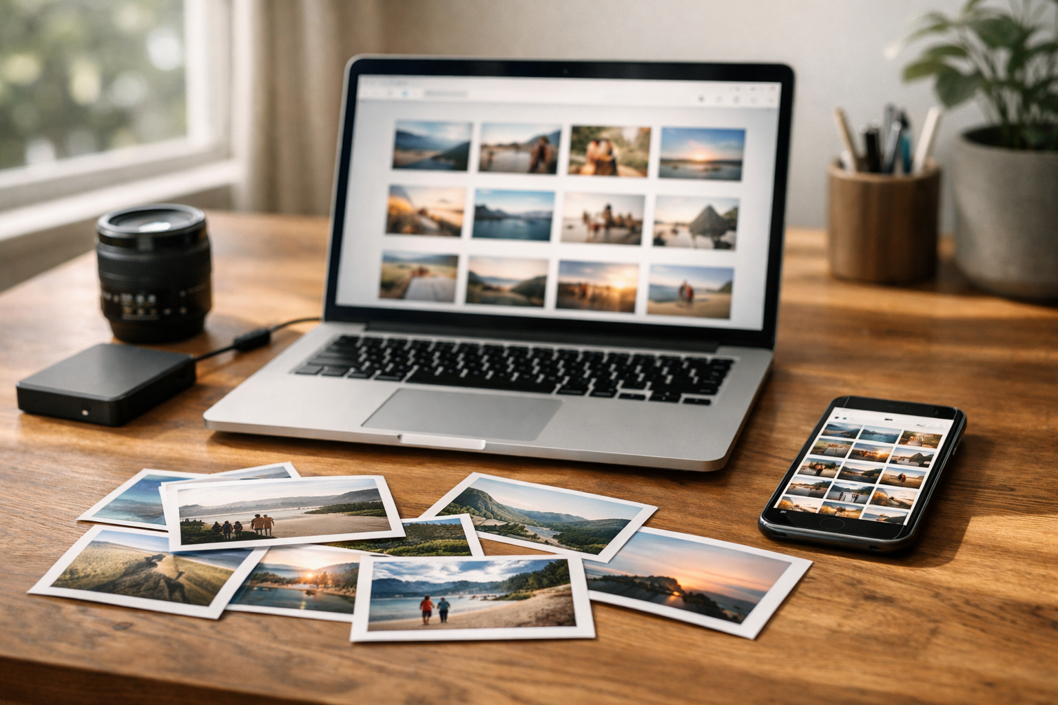
Turn your photo folder into a searchable library using Image AI.
This beginner-friendly course is a short, book-style walkthrough that helps you create an Image AI visual search tool for your personal photo library. Instead of searching by filenames or manually added tags, you’ll learn how to search by “looks like.” That means you can pick one photo (a beach shot, a pet photo, a birthday picture) and instantly retrieve other photos that feel visually similar.
You don’t need to know coding, math, or data science to begin. We’ll start from first principles and use a pretrained model (a model that has already learned from large image collections) so you can get strong results without training anything yourself.
You’ll create a simple, local tool that can:
This project is designed for real life: messy folders, mixed file types, and the need to keep personal images private.
Each chapter builds on the last. First you’ll understand the idea behind visual similarity in plain language. Then you’ll set up your workspace and learn how to load images reliably. Next, you’ll generate embeddings using a pretrained model and confirm they behave as expected. After that, you’ll build the actual search step (finding the nearest matches). Finally, you’ll wrap everything in a small app-like interface, and finish with quality checks, privacy practices, and packaging so you can reuse your tool later.
Many AI tutorials jump straight into complex training or heavy math. This course does the opposite: you’ll focus on the minimum concepts needed to build something useful. You’ll learn what an embedding is, why distance measures similarity, and how an index makes searching fast. Every concept is tied directly to a concrete step in your project, so the learning feels practical instead of abstract.
Because you’re working with personal photos, you’ll learn safe habits early: working from a copied folder, avoiding accidental sharing, and keeping the tool local-first. You’ll also learn how to structure your project so it’s easy to delete, rebuild, or move without losing control of your data.
If you’re ready to turn your photo folder into a searchable visual library, you can begin today. Register free to access the course, or browse all courses to explore related beginner paths.
Machine Learning Engineer, Computer Vision
Sofia Chen builds practical computer vision systems for search and media organization. She specializes in beginner-friendly workflows that turn AI concepts into working tools. Her teaching focuses on clear mental models, safe data handling, and small wins that stack into real projects.
Most photo libraries are searchable only by what you remembered to type: filenames, folders, dates, or a few tags. That works until you need “the photo where the dog is on the couch” or “pictures that look like this sunset,” and you don’t know what anything was named. This course is about building a different kind of search: visual search—finding images by how they look.
In this chapter, you’ll get the mental model that makes the rest of the project feel straightforward: we turn each image into a compact numeric representation (an embedding), store those numbers in an index, and then do fast similarity search to return the nearest matches. No model training is required; we’ll rely on a pre-trained vision model that already understands many visual patterns. You’ll also set up a safe practice photo library, because good engineering starts with good data hygiene.
By the end of Chapter 1 you should be able to describe the goal (“search by looks like”), explain embeddings and similarity, outline the full pipeline end-to-end, and prepare a personal photo folder in a way that minimizes risk and maximizes reproducibility.
Practice note for Milestone: Understand the goal—search by “looks like,” not filenames: document your objective, define a measurable success check, and run a small experiment before scaling. Capture what changed, why it changed, and what you would test next. This discipline improves reliability and makes your learning transferable to future projects.
Practice note for Milestone: Learn the core idea of similarity using vectors (intuitive): document your objective, define a measurable success check, and run a small experiment before scaling. Capture what changed, why it changed, and what you would test next. This discipline improves reliability and makes your learning transferable to future projects.
Practice note for Milestone: Map the full project pipeline from photos to results: document your objective, define a measurable success check, and run a small experiment before scaling. Capture what changed, why it changed, and what you would test next. This discipline improves reliability and makes your learning transferable to future projects.
Practice note for Milestone: Set up a safe practice photo library (copy + organize): document your objective, define a measurable success check, and run a small experiment before scaling. Capture what changed, why it changed, and what you would test next. This discipline improves reliability and makes your learning transferable to future projects.
Practice note for Milestone: Understand the goal—search by “looks like,” not filenames: document your objective, define a measurable success check, and run a small experiment before scaling. Capture what changed, why it changed, and what you would test next. This discipline improves reliability and makes your learning transferable to future projects.
Visual search means you provide an image (or sometimes a text description) and the system returns other images that are visually similar. The key milestone is understanding the goal: you’re searching by “looks like,” not by filenames or manual tags. In a personal photo library, this solves problems like: “find other photos from this hike,” “find images with a similar composition,” or “show me pictures that look like this person’s face from another day.”
Tag-based search is different. Tags are discrete labels (e.g., beach, birthday, dog) that must be created or predicted. Tagging can be powerful, but it is brittle: it depends on vocabulary, misses nuance, and often fails when you didn’t tag consistently. Visual search is continuous: it doesn’t require you to pre-decide categories; instead it retrieves “nearby” images in a visual feature space.
Engineering judgment: don’t treat visual search as a replacement for everything. It’s best when you have a reference image and want more like it. It’s less direct for precise queries like “photos from March 2022” unless you combine it with metadata filtering. A common mistake is expecting visual search to read your mind; you still need to define what “similar” should mean for your use case (scene similarity, object similarity, faces, colors, etc.). In this course, we’ll start with general similarity and learn how to tighten results later.
Computers see an image as a grid of pixels. Each pixel is a small set of numbers (for example, RGB values). If you take two photos and compare them pixel-by-pixel, you’ll quickly discover why raw pixels are a poor basis for visual search: small shifts, different lighting, resizing, or compression can change many pixels even when the photo “means the same thing” to a human.
This section’s milestone is building intuition: there are two levels of “image as numbers.” The first is pixels (low-level measurements). The second is meaning (higher-level patterns such as edges, textures, object parts, and overall scene layout). Good visual search needs numbers that are stable under normal variations: a dog is still a dog if the photo is brighter, cropped slightly, or taken from a different angle.
Practical outcome: when you implement your pipeline later, you will resize images to a consistent input size because the model expects it, but you won’t rely on resized pixels for matching. Another common mistake is mixing file formats and color spaces without noticing. For example, some images may be CMYK, grayscale, or have an embedded color profile. A robust ingestion step standardizes to RGB and handles corrupted files gracefully (skip, log, continue) instead of crashing halfway through your library.
An embedding is a vector (a list of numbers) produced by a neural network that summarizes an image in a compact, meaningful way. Think of it as a “fingerprint,” but not a unique ID; rather, it’s a coordinate in a feature space where similar images land near each other. This is the core concept that enables visual search.
Here’s the practical idea: you run each photo through a pre-trained vision model (no training needed), and the model outputs a vector like [0.12, -0.03, ...] with perhaps 512, 768, or 1024 dimensions. You store that vector along with a pointer to the original file (path, filename, or an internal ID). Later, when you query with a new image, you generate its embedding and find the closest stored vectors.
Engineering judgment: embeddings are not “truth.” They reflect what the model learned from its training data and objectives. A common mistake is assuming the embedding is perfect for faces, private environments, or niche domains. Another mistake is changing the model mid-project; embeddings from different models are not directly comparable, so you should pick one model and stick with it for a given index. In later chapters you’ll learn to re-embed safely if you decide to upgrade.
Once images are embeddings (vectors), similarity search becomes a geometry problem: find which vectors are closest to a query vector. The most common tools are cosine similarity (angle between vectors) and Euclidean distance (straight-line distance). Many modern embedding models are designed so cosine similarity works well, often after normalizing vectors to length 1.
The milestone here is learning similarity intuitively. Imagine each image as a point in a high-dimensional space. You can’t visualize 512 dimensions, but you can rely on a simple rule: points that represent similar images cluster together. A query is just “drop a point into the space and retrieve its nearest neighbors.”
Common mistakes: (1) forgetting to normalize when your similarity metric expects it, leading to unstable rankings; (2) comparing vectors with different dimensions (usually due to mixing models); (3) evaluating only “one good demo query” instead of a small set of representative queries. Practical outcome: you will later evaluate results by trying multiple queries—people, pets, landscapes, indoor scenes—and checking whether the top results are consistent and diverse. If results feel off, you’ll have levers: choose a different model, adjust preprocessing, or clean duplicates and near-identical bursts of photos that can dominate the top results.
Before writing code, map the full pipeline. This milestone helps you avoid the beginner trap of building a UI first and discovering later that your data handling is unsafe or your embeddings aren’t reproducible. Our pipeline has four stages, each with clear inputs/outputs and failure modes you can test.
(image_id, embedding_vector).Engineering judgment: prioritize repeatability. If you can’t reproduce the same index tomorrow, debugging becomes painful. Store: model name/version, preprocessing steps (image size, normalization), and the mapping from index rows to file paths. Common mistakes include indexing absolute paths that later change (breaking results) and forgetting to handle deletions or moved files. A practical approach for personal projects is to copy photos into a dedicated “library” folder and index relative paths within that folder, so the project is portable and less fragile.
This blueprint also clarifies what “fast search” means: embedding is the expensive step; searching vectors is comparatively cheap, especially once indexed. That’s why we embed the library once, save the index, and reuse it for many queries.
Working with personal photos requires a safety-first setup. This milestone is about preparing a practice library without risking data loss, accidental sharing, or leaking sensitive information. Even if your code runs locally, mistakes happen: deleting originals, uploading logs, or accidentally committing file paths into a public repository.
Start by creating a dedicated project workspace with a clear separation between originals and working copies. Do not point your ingestion script at your only copy of family photos. Instead, make a copy of a small subset (for example 200–2000 images) into a folder like photo_search_library/. Keep the original folder read-only, or simply never touch it with code.
Common mistakes: committing sample photos to GitHub, embedding private filenames into screenshots, or storing indices in shared cloud folders. Practical safeguards: add your library folder and index files to .gitignore, keep logs free of full paths when possible, and verify your app doesn’t automatically upload anything. If you later choose to run embeddings with a hosted API, treat that as data sharing and review terms and policies carefully. For this course, we’ll keep the first version local so you can learn the concepts while staying in control of your data.
1. What is the main goal of the visual search system described in Chapter 1?
2. In this chapter’s mental model, what is an image embedding used for?
3. Which sequence best matches the end-to-end pipeline described for visual search?
4. Why does Chapter 1 emphasize that no model training is required?
5. What is the main reason for setting up a safe practice photo library (copy + organize) before building the system?
This chapter gets you from “I have a folder of photos” to “I can run a script that reads them, prepares them consistently, and saves useful outputs.” In Chapter 1 you learned the core idea: an image embedding is a compact numeric “fingerprint” produced by a pre-trained model. Visual search becomes possible because “similar” images tend to land near each other in embedding space, so searching is just “find the nearest vectors.”
Now we’ll build the practical foundation for that workflow. Before worrying about fancy user interfaces or databases, you’ll set up a safe project folder, install the minimum tools, and run a small “hello project” script that proves your environment can read images and write results. Then you’ll add each step you need later: loading images carefully (including handling broken files), resizing and normalization (to keep embeddings consistent), batch processing (so you can process hundreds or thousands of photos), and saving metadata plus embeddings to disk in a clean structure.
The engineering judgment to practice here is simple: build a reliable pipeline first. Visual search quality is often limited not by the model, but by inconsistency in preprocessing, silent failures (skipped images), and messy outputs that are hard to debug. Treat this chapter as laying track for everything that follows.
Practice note for Milestone: Install the tools and run a “hello project” check: document your objective, define a measurable success check, and run a small experiment before scaling. Capture what changed, why it changed, and what you would test next. This discipline improves reliability and makes your learning transferable to future projects.
Practice note for Milestone: Load and preview images from a folder: document your objective, define a measurable success check, and run a small experiment before scaling. Capture what changed, why it changed, and what you would test next. This discipline improves reliability and makes your learning transferable to future projects.
Practice note for Milestone: Write a script that processes a batch of photos: document your objective, define a measurable success check, and run a small experiment before scaling. Capture what changed, why it changed, and what you would test next. This discipline improves reliability and makes your learning transferable to future projects.
Practice note for Milestone: Save outputs to disk in a clean project structure: document your objective, define a measurable success check, and run a small experiment before scaling. Capture what changed, why it changed, and what you would test next. This discipline improves reliability and makes your learning transferable to future projects.
Practice note for Milestone: Install the tools and run a “hello project” check: document your objective, define a measurable success check, and run a small experiment before scaling. Capture what changed, why it changed, and what you would test next. This discipline improves reliability and makes your learning transferable to future projects.
Your goal in this milestone is to install a small, stable toolset that lets you run a complete end-to-end “hello project” check: load an image, transform it, and save a result to disk. Keep the stack minimal so debugging stays easy.
Python. Use a recent Python 3 release that your OS supports well (for many learners this means Python 3.10–3.12). Create an isolated environment (venv or conda) so package versions don’t collide with other projects. A dedicated environment matters because computer vision libraries often depend on compiled wheels; mixing versions can produce confusing import errors.
Core packages. For this chapter you need: (1) an image library (Pillow is beginner-friendly), (2) a numerical array library (NumPy), (3) a progress indicator (tqdm), and (4) your embedding model stack. If you’ll use a pre-trained model like CLIP via PyTorch, install torch/torchvision plus the model wrapper you choose. If you prefer a lightweight embedding model through a library like sentence-transformers (which can also host CLIP variants), install that instead. The key is: no training, just inference.
Folders. Create a project directory that contains code, configuration, inputs, and outputs. Do not point scripts at your only copy of personal photos. Make a copy of a small subset (e.g., 50–200 images) to learn with. This is a privacy and safety step: you’ll avoid accidentally uploading, modifying timestamps, or generating derived files in your original library.
Hello project check. Write a tiny script that prints your Python version, imports all packages, reads one image, and writes a resized preview to an outputs folder. If this runs cleanly, you’ve proven the environment works before you add the complexity of embeddings and indexing.
A clean project layout is not bureaucracy; it is the difference between a repeatable pipeline and a one-off experiment. Visual search systems involve many derived artifacts: resized images, embeddings, indexes, and metadata tables. If you don’t separate inputs from outputs, you will eventually overwrite something important or lose track of which embeddings correspond to which preprocessing settings.
Use a structure like this (adapt as needed):
Configuration matters early. Beginners often hardcode paths like C:\Users\... into scripts. That works once, then breaks. Put key settings into a config file (JSON/YAML/TOML) or a small Python settings.py: input folder path, output folder path, image size, model name, batch size. This also makes later evaluation easier because you can record which configuration produced which results.
Privacy and safety. Keep inputs as copies, and avoid writing anything into the input tree. If you later build a UI, store search results and thumbnails in outputs/ or data/derived/. This habit reduces the chance of leaking personal data into source control. Add your data/ directory to .gitignore from the start, so you don’t accidentally commit private images or embeddings.
This milestone connects directly to “save outputs to disk in a clean project structure.” If you can run your script twice and get the same derived outputs in the same places, you are building a reliable foundation for the visual search app you’ll create later.
Loading photos sounds trivial until you meet real photo libraries: mixed formats, giant files, partial downloads, and images with odd metadata. Your batch script must be defensive. A single corrupted file should not crash a 5,000-image run.
Supported formats. Start with JPG/JPEG and PNG. Many phone libraries also contain HEIC/HEIF. Pillow may not read HEIC without extra plugins, so decide early: either (a) convert HEIC to JPEG outside your pipeline for now, or (b) install the needed decoder. For a beginner-friendly path, keep your first dataset to formats your loader handles reliably. You can expand later.
Corrupted files and exceptions. Wrap image loading in try/except. When a load fails, record it (filename + error) into a log or a “skipped.csv” file and continue. This is essential for debugging and for “cleaning” your library later. A common mistake is to silently skip failures without tracking them; then you wonder why some photos never appear in search.
Color modes. Images may be RGB, grayscale, palette-based, or include alpha (RGBA). Most embedding models expect 3-channel RGB. Convert consistently: img = img.convert('RGB'). If you forget this, you might get shape mismatches or inconsistent embeddings.
Orientation metadata. Many phone photos rely on EXIF orientation. If you ignore it, images may be rotated incorrectly, and embeddings will reflect that. Decide on a standard approach: apply EXIF transpose at load time so the pixels match how the photo appears in viewers.
Preview milestone. As part of “load and preview images from a folder,” make a small preview grid or save a few thumbnails to outputs/previews/. This isn’t about aesthetics; it’s a sanity check that your loader is reading the right files, in the right orientation, and with the expected colors.
Embeddings are only comparable if the model sees images prepared in the same way every time. That means consistent resizing and consistent normalization. This section is where many “my search results are random” problems actually begin.
Resize strategy. Most pre-trained vision models expect a fixed input size (for example 224×224). You have options: (1) center-crop after resizing the shorter side, (2) resize directly (which can distort), or (3) pad to square (“letterbox”). For personal photo search, center-crop is a common default because it preserves scale and keeps the model’s expected composition. However, it can cut off important content at the edges (a person near the border). If you notice missed matches later, revisit this choice.
Interpolation. Use a reasonable resampling method (bilinear/bicubic). Nearest-neighbor can create artifacts that slightly change embeddings. The goal is not perfect image quality, but stable model input.
Normalization. Models typically expect pixel values scaled to [0,1] and then normalized with channel-wise mean/std values specific to the model’s training (e.g., ImageNet stats). If you skip normalization or use the wrong values, embeddings can be systematically shifted, reducing similarity accuracy. Follow the model’s documentation and treat preprocessing as part of the model, not an optional step.
Determinism. Ensure the same image always produces the same embedding. Turn off random augmentations. Use the model in evaluation/inference mode. If your pipeline includes any randomness, you will store embeddings that don’t reproduce later, making debugging painful.
Practical outcome: at the end of this milestone, you should be able to take one image, apply your preprocessing, feed it into the pre-trained model, and obtain a fixed-length embedding vector. You are not building the full search yet, but you are guaranteeing that whatever you store in your index will be consistent across runs.
This milestone is where your project becomes real: you’ll write a script that processes a batch of photos and produces embeddings for all of them. The core pattern is: list files → for each file: load → preprocess → embed → store results → continue even on errors.
File discovery. Use a recursive scan so subfolders work. Filter by extension, but don’t rely on extensions alone—some files may be mislabeled. Keep a clear count: “Found N candidate images.” That number should match your expectations for the folder you copied.
Progress and observability. Wrap the loop with tqdm so you can see throughput and remaining time. Also print (or log) periodic summaries: processed, skipped, average time per image. Beginners often run a script with no output for five minutes and assume it’s frozen.
Speed basics. Without over-optimizing, a few choices matter:
Common mistakes. The biggest is mixing concerns: embedding code that also writes UI outputs, thumbnails, and debug plots. Keep the batch embedding script focused. It should do one job well: produce a reliable set of embeddings and metadata that later components can consume.
Practical outcome: you can point the script at data/input_photos/ and get a complete run that finishes, reports what happened, and leaves artifacts you can inspect.
Embeddings alone are not useful unless you can map each vector back to the original photo. That mapping is metadata: a stable ID, the file path, and any other fields you’ll want for search results. Treat metadata as a first-class output of your pipeline.
Choose an ID scheme. A simple approach is an incrementing integer ID assigned in the order you process files. A more stable approach is to compute a content hash (e.g., SHA-1 of the file bytes) so duplicates and renames are handled gracefully. For a beginner project, start with integer IDs plus the relative path; add hashing later if you find many duplicates.
Save a table. Write a CSV or Parquet file with columns like: id, relative_path, width, height, status, error. If you skip an image, record why. This table becomes your single source of truth when your search app needs to display results and when you want to clean the dataset.
Save embeddings. For a simple local index, you can store embeddings as a NumPy array file (.npy) aligned by row with the metadata table. Example: row 17 in embeddings.npy corresponds to id=17 in your CSV. Keep the embedding dimensionality consistent; if you switch models, store in a new folder (e.g., data/index/clip_vit_b32/) to avoid mixing incompatible vectors.
Engineering judgment: version your outputs. If you change preprocessing (crop strategy, image size, normalization), the embeddings change. Record these settings in a small index_config.json saved alongside the embeddings and metadata. Later, when you evaluate search results, you’ll be able to say “this index was created with center-crop at 224 and model X.” Without this, improvements become guesswork.
Practical outcome: after this milestone, your project has a repeatable disk representation of your photo library for visual search—images remain untouched, and derived artifacts (metadata + embeddings) live in a well-defined output structure ready for similarity search in the next chapter.
1. What is the main goal of Chapter 2 in the visual search workflow?
2. Why does the chapter emphasize resizing and normalization before generating embeddings?
3. Which situation is the chapter warning you to handle explicitly when loading images from a folder?
4. Why is batch processing an important milestone in this chapter?
5. What is the practical reason for saving metadata and embeddings to disk in a clean project structure?
In Chapter 2 you organized your photos and clarified what “similar” should mean for your personal visual search (same person, same place, same event, same object, etc.). In this chapter you’ll build the core representation that makes visual search practical: image embeddings. An embedding is a fixed-length vector (a list of numbers) that summarizes what a model “sees” in an image. Once every photo becomes a vector, finding similar photos becomes a fast math problem: compare vectors and return the closest ones.
You will not train any neural network in this chapter. Instead, you’ll use a pretrained model—a model already trained on a large dataset—to turn your photos into embeddings. This gives you a huge capability boost with beginner-friendly effort: load a model, preprocess an image, run inference, and store the resulting vector alongside the photo’s ID.
The engineering focus here is building a reliable pipeline. You’ll create embeddings consistently (same preprocessing each time), store them safely (so you don’t lose work), and verify they behave as expected. By the end, you’ll have four practical milestones completed: (1) use a pretrained model to convert images to embeddings, (2) store embeddings next to photo IDs, (3) verify embeddings are stable and usable, and (4) implement a simple similarity check between two photos.
Throughout this chapter, assume you’re working on copies of your photo folder, not originals, and that you avoid uploading personal images to third-party services unless you explicitly decide to. A local workflow (Python + a pretrained model on your machine) is a good default for privacy.
Practice note for Milestone: Use a pretrained model to turn photos into embeddings: document your objective, define a measurable success check, and run a small experiment before scaling. Capture what changed, why it changed, and what you would test next. This discipline improves reliability and makes your learning transferable to future projects.
Practice note for Milestone: Store embeddings alongside photo IDs: document your objective, define a measurable success check, and run a small experiment before scaling. Capture what changed, why it changed, and what you would test next. This discipline improves reliability and makes your learning transferable to future projects.
Practice note for Milestone: Verify embeddings are consistent and usable: document your objective, define a measurable success check, and run a small experiment before scaling. Capture what changed, why it changed, and what you would test next. This discipline improves reliability and makes your learning transferable to future projects.
Practice note for Milestone: Build a simple “similarity check” between two photos: document your objective, define a measurable success check, and run a small experiment before scaling. Capture what changed, why it changed, and what you would test next. This discipline improves reliability and makes your learning transferable to future projects.
Practice note for Milestone: Use a pretrained model to turn photos into embeddings: document your objective, define a measurable success check, and run a small experiment before scaling. Capture what changed, why it changed, and what you would test next. This discipline improves reliability and makes your learning transferable to future projects.
Practice note for Milestone: Store embeddings alongside photo IDs: document your objective, define a measurable success check, and run a small experiment before scaling. Capture what changed, why it changed, and what you would test next. This discipline improves reliability and makes your learning transferable to future projects.
Practice note for Milestone: Verify embeddings are consistent and usable: document your objective, define a measurable success check, and run a small experiment before scaling. Capture what changed, why it changed, and what you would test next. This discipline improves reliability and makes your learning transferable to future projects.
A pretrained model is a neural network that has already learned general visual features from a large dataset. For you, that means you can use it immediately as a feature extractor: feed in an image and receive an embedding vector. No labels, no GPUs, and no training loop are required. This is the fastest way to start a personal photo visual search project because the heavy learning has been done ahead of time.
It helps to separate two activities: training (teaching a model by adjusting its weights) and inference (running a trained model to get outputs). In this chapter you only do inference. Your “model improvement” comes from better data hygiene (cleaner folders, consistent inputs) and better indexing/search logic—not from modifying the model weights.
Workflow-wise, “use a pretrained model” usually looks like: (1) load weights from a trusted library, (2) apply the model’s required image preprocessing (resize, crop, normalize), (3) run a forward pass, and (4) capture the embedding output. You then store the embedding along with a stable photo identifier. This is your first milestone: turn photos into embeddings.
Common mistakes at this stage are operational, not mathematical: using different preprocessing in different runs, silently failing to read certain file types, or embedding edited copies without realizing it. Treat your embedding pipeline as a reproducible process: log the model name/version, record preprocessing parameters, and keep your photo IDs stable so you can always trace an embedding back to the exact file.
For beginner-friendly visual search, you want a model that produces robust embeddings across everyday photos: people, pets, landscapes, indoor scenes, screenshots, and a wide range of lighting. A practical choice is a CLIP-style image encoder (or a similar general-purpose embedding model). The intuition: these models were trained to align images with language, so they learn high-level semantics (e.g., “dog on a beach,” “birthday cake,” “mountain skyline”) instead of only low-level texture.
In practice, this tends to make search results feel more “human”: a query photo of a bicycle might bring back other bicycle photos even if colors differ. That semantic robustness is valuable for personal libraries where compositions and lighting vary. For your app, you only need the image encoder portion—no text prompts required to compute embeddings for similarity search.
Engineering judgement: pick one model and stick with it for a while. Mixing models in the same index is usually a mistake because embeddings from different encoders are not comparable. If you do change models later, rebuild the index from scratch and store the model metadata with the embeddings so you can reproduce results.
Finally, remember the goal is not “best benchmark accuracy.” Your goal is a dependable embedding that makes your similarity search useful on your personal photos. Start simple, validate results, then tune later.
Generating embeddings is a repeatable pipeline: load image → preprocess → encode → store. The model expects inputs with a specific shape and value range. Most vision encoders operate on a batch of images shaped like [batch, channels, height, width] (often called NCHW). Channels are usually 3 (RGB). Height and width depend on the model (commonly 224×224 or similar). Even if your photo is 4032×3024, you will resize/crop it to the model’s expected size.
The output is an embedding tensor shaped like [batch, d], where d is the embedding dimension (for example 512, 768, or 1024). For a single image, you can treat it as a 1D vector of length d. This vector is your photo’s “signature” for similarity comparisons.
To keep things consistent, define a function that takes a file path and returns: (1) a stable photo_id and (2) the embedding vector. A good photo_id can be the relative path inside your dataset folder (e.g., 2023/Trip/IMG_1042.jpg) or a hash of the file contents if you want immutability. This is your second milestone: store embeddings alongside photo IDs.
Make a small “embedding run” on 20–50 photos first. Print shapes, confirm no exceptions, and inspect a few embeddings for obvious anomalies (e.g., all zeros or NaNs). This is part of the third milestone: verify embeddings are consistent and usable before committing to embedding your whole library.
Once you have embeddings, you need a comparison rule. The most common beginner-friendly approach is cosine similarity: it measures the angle between vectors, not their raw magnitude. However, cosine similarity is simplest when you first L2-normalize each embedding (scale it to length 1). After normalization, cosine similarity between two vectors becomes just their dot product, which is fast and numerically stable.
Why normalization matters: raw embeddings can vary in magnitude for reasons unrelated to content (model internals, preprocessing differences, or batch effects). If you compare unnormalized vectors with Euclidean distance, you can accidentally rank images by “vector length” rather than actual semantic closeness. Normalizing makes your similarity measure more consistent across different photos and runs.
e_norm = e / (||e|| + 1e-12)sim(a,b) = a_norm · b_norm (ranges roughly from -1 to 1)1 - sim for “smaller is closer” sortingEngineering judgement: normalize once at embedding creation time and store the normalized vector. This avoids repeating work at query time and reduces the chance that you forget to normalize in one code path. If you later want to experiment (e.g., using Euclidean distance), keep a flag in your metadata describing the normalization so your index stays coherent.
This section connects directly to your fourth milestone: building a simple similarity check between two photos. If the vectors are normalized, the check can be a single dot product and a threshold you can reason about (for example, “above 0.30 often feels similar” depends on the model and dataset).
Embeddings are only useful if you can reuse them without recomputing every time. Your goal is a simple local index: a table of photo_id plus an array of embeddings. For beginners, two practical storage approaches are (1) NumPy files for the numeric matrix and (2) a small JSON (or CSV) file for IDs and metadata.
A common pattern:
[N, d] (fast to load and compute with)N IDs aligned by index with the rows in embeddings.npyThis alignment requirement is critical: row i in the embedding matrix must always refer to photo_ids[i]. Most “my search results are wrong” bugs come from broken alignment after filtering, sorting, or partial re-embedding. When you add new photos later, append to both structures together, or rebuild the entire index to be safe.
JSON is human-readable but inefficient for large vectors. Avoid storing full embeddings as JSON arrays unless your dataset is tiny; it bloats file size and loads slowly. Use NumPy (.npy or .npz) for vectors and JSON only for IDs/metadata. When loading, validate shapes: confirm the number of IDs equals N, confirm d matches your current model, and confirm the dtype is float32 (or float16 if you intentionally optimized memory).
With these files in place, your “search app” can start instantly: load embeddings and IDs, compute a query embedding for one input photo, compare it against the matrix, and return the nearest photo IDs to display.
Before you trust your visual search results, run a few sanity tests. These checks catch the most common pipeline failures early and give you intuition for what the model considers “similar.” They also complete the milestone of verifying embeddings are consistent and usable.
Next, do a small “top-k neighbors” inspection. Choose 5–10 query photos and retrieve the top 10 most similar items from your index. Look for patterns: are results grouped by event (good), by color palette (sometimes okay), or by repetitive textures (sometimes a warning sign)? Odd results often come from non-photo images in your dataset—screenshots, memes, scanned documents, or tiny thumbnails. You can improve search by filtering file types, removing corrupted images, and excluding extremely small resolutions.
Finally, implement a beginner-friendly two-photo similarity check: select photo A and photo B, compute their embeddings, normalize, and print a similarity score. This tiny tool is surprisingly powerful for debugging. If you can’t make the two-photo check behave sensibly, your full search app will not behave sensibly either. Once the sanity tests pass, you are ready to scale to your whole folder and build the “return similar photos” experience on top of your embedding index.
1. Why do image embeddings make visual search practical in this chapter’s approach?
2. What is the main reason the chapter emphasizes using a pretrained model rather than training a new one?
3. Which engineering practice is most important for producing consistent, usable embeddings?
4. What does it mean to “store embeddings alongside photo IDs,” and why does it matter?
5. Which scenario best reflects a common cause of incorrect similarity results mentioned in the chapter?
In earlier chapters you prepared a folder of photos and learned how to turn each image into a numeric “fingerprint” called an embedding. This chapter is where those embeddings become a usable tool: a visual search engine that can take one photo as a query and return the most similar photos from your library. The core idea is simple: if two images “look alike,” their embeddings should end up close together in a vector space. Your job is to store those vectors safely and search them quickly.
We will build the engine in four practical milestones that map to real product behavior. First, you will create a nearest-neighbor search over your library—meaning you can find the closest embedding vectors to a query vector. Second, you will return top-K results for a chosen query image, with clear rules (like not returning the query image itself). Third, you’ll add basic performance improvements so the tool stays responsive as your photo folder grows. Finally, you’ll produce a clean results page in a grid so you can inspect matches visually and decide what to improve.
Throughout, keep a beginner-friendly mindset: prefer a local index (a file on your machine), deterministic behavior, and small, testable pieces. You don’t need training, GPUs, or cloud services. You do need engineering judgment: consistent preprocessing, careful handling of filenames, and a willingness to debug why certain “bad matches” happen. By the end of this chapter you will have a working app that answers a concrete question: “Show me photos similar to this one.”
The rest of the chapter walks through each decision: what indexing means, which similarity metric to use, how to store and query embeddings locally, how to format results, and how to troubleshoot. Treat it like you’re building a small “search feature” you could realistically keep and maintain.
Practice note for Milestone: Create a nearest-neighbor search over your library: document your objective, define a measurable success check, and run a small experiment before scaling. Capture what changed, why it changed, and what you would test next. This discipline improves reliability and makes your learning transferable to future projects.
Practice note for Milestone: Return top-K results for a chosen query image: document your objective, define a measurable success check, and run a small experiment before scaling. Capture what changed, why it changed, and what you would test next. This discipline improves reliability and makes your learning transferable to future projects.
Practice note for Milestone: Add basic performance improvements for larger folders: document your objective, define a measurable success check, and run a small experiment before scaling. Capture what changed, why it changed, and what you would test next. This discipline improves reliability and makes your learning transferable to future projects.
Practice note for Milestone: Produce a clean results page (grid) for inspection: document your objective, define a measurable success check, and run a small experiment before scaling. Capture what changed, why it changed, and what you would test next. This discipline improves reliability and makes your learning transferable to future projects.
Practice note for Milestone: Create a nearest-neighbor search over your library: document your objective, define a measurable success check, and run a small experiment before scaling. Capture what changed, why it changed, and what you would test next. This discipline improves reliability and makes your learning transferable to future projects.
Practice note for Milestone: Return top-K results for a chosen query image: document your objective, define a measurable success check, and run a small experiment before scaling. Capture what changed, why it changed, and what you would test next. This discipline improves reliability and makes your learning transferable to future projects.
Practice note for Milestone: Add basic performance improvements for larger folders: document your objective, define a measurable success check, and run a small experiment before scaling. Capture what changed, why it changed, and what you would test next. This discipline improves reliability and makes your learning transferable to future projects.
Indexing is the step where you organize your stored embeddings so you can search them efficiently. Without an index, the simplest approach is “brute force”: compute the distance from the query embedding to every photo embedding and sort the results. Brute force is perfectly fine for a few hundred photos and is often the best place to start because it is easy to implement and easy to verify.
The moment your library grows to thousands or tens of thousands of photos, brute force starts to feel slow, especially if you’re building a small UI and want results in under a second. That’s when indexing matters. An index is a data structure that helps you find nearest neighbors without comparing against every vector. Conceptually, it narrows the search to likely candidates and avoids unnecessary computations.
For this chapter’s milestones, think of indexing in two levels:
Common mistake: rebuilding embeddings every time you search. Indexing implies a “build once, query many times” workflow. You should generate embeddings once, save them, and reload them quickly on app start. Another common mistake is losing the mapping between embedding rows and filenames. Your index is only useful if you can reliably go from “row 1234” back to “IMG_1234.jpg”. Keep a parallel list (or a small table) of file paths aligned with the embedding matrix.
Milestone connection: when you “create a nearest-neighbor search over your library,” you are really creating your first index—maybe just an embeddings matrix and a list of file paths. That alone can feel like magic: choose one photo, and the library responds with visually similar items.
Nearest-neighbor search requires a definition of “close.” Two common choices are cosine similarity and Euclidean distance. The good news: you can build a working search engine with either. The better news: for many modern embedding models, one option is typically more stable.
Cosine similarity measures the angle between vectors. If two embeddings point in the same direction, cosine similarity is high—even if one vector has a larger magnitude. In plain language: cosine asks, “Do these two photos have similar patterns of features?” rather than “Are the numbers the same size?” This is often a good default because embeddings can vary in magnitude for reasons unrelated to image content (model specifics, preprocessing differences, etc.).
Euclidean distance measures straight-line distance in the embedding space. It treats magnitude as meaningful: if the vector lengths differ, the distance increases. Euclidean is intuitive and works well when embeddings are already normalized or when the model was designed for Euclidean comparisons.
A practical rule you can apply immediately:
Common mistake: mixing metrics between indexing and querying. If you build an ANN index configured for Euclidean distance but later interpret scores as cosine similarity, your results will look inconsistent and confusing. Decide on one metric, document it, and keep it consistent end-to-end (embedding normalization, index configuration, query scoring, and displayed scores).
Milestone connection: when you “return top-K results,” the metric affects what “top” means. With cosine, top-K means highest similarity scores; with Euclidean, top-K means smallest distances. Keep your UI wording accurate so you don’t misread your own results.
A beginner-friendly local index can be built from two files: (1) an embeddings array and (2) metadata that maps each row to a photo. This is enough to satisfy the first milestone: a nearest-neighbor search over your library.
Start with a folder scan that collects stable identifiers for each image. Prefer absolute paths or paths relative to a chosen “library root.” Store them exactly as you will use them later. Then generate embeddings using your pre-trained model and store them in the same order as the file list. Finally, write them to disk.
.npy (NumPy) file, or .npz if you want compression..json file containing an array of records (path, file size, modified time) or a CSV with path + index.Why store file size and modified time? Because personal photo libraries change. If a user replaces a photo, moves folders, or edits files, you need a way to detect that your index is stale. A minimal approach is: on startup, compare current file count and (path, mtime) pairs to what you stored. If anything differs, rebuild embeddings for the changed files (or rebuild the index entirely at first, then optimize later).
For performance, even a brute-force search can be fast if you do it correctly. Load embeddings into a 2D float32 matrix once. Normalize embeddings if using cosine. Then compute similarity using vectorized operations rather than Python loops. This one decision—vectorization—can be the difference between “works but slow” and “feels instant.”
Common mistake: silently skipping images that fail to load and ending up with misaligned arrays. If an image fails, record it explicitly (log a warning, add it to a “skipped” list) and do not add a placeholder vector unless you also add a placeholder filename in the same position. Alignment is everything in a simple index.
Milestone connection: after this step, you have a durable local index: embeddings + filenames. That is the core artifact your search engine depends on.
Querying is the moment your system behaves like a search engine. The workflow is: (1) pick a query image, (2) compute its embedding using the same preprocessing and model used for the library, (3) compare it to the index embeddings, and (4) return the best matches.
Top-K is the simplest, most user-friendly output: return the K most similar photos. K=10 or K=20 is a good default for inspection. Implementing top-K efficiently matters: rather than sorting all N scores, you can use a partial selection (for example, argpartition in NumPy) and then sort just the top slice. That small change is one of the easiest “basic performance improvements” you can make as folders grow.
Thresholds help avoid showing garbage results. For cosine similarity, you might decide that anything below 0.20 (example only) is “not similar enough” and should be omitted or displayed in a separate section. Thresholds are highly model- and dataset-dependent, so treat them as a tunable setting rather than a fixed rule.
Exclude the same image is more important than it sounds. If the query image is from the same folder, the nearest neighbor will often be the query itself (identical file path) or a duplicate (same photo resized). Your search results feel much smarter when you explicitly filter these cases:
Common mistake: inconsistent preprocessing at query time. If you resized library images to 224×224 with center-crop but query images with a different resize strategy, your similarity scores can degrade noticeably. Lock down a single preprocessing function and reuse it for both indexing and querying.
Milestone connection: this section completes “Return top-K results for a chosen query image.” Once you see top-K working reliably, you can begin evaluating quality and tuning thresholds, K, and filtering rules.
A search engine is only as useful as its output. If you only print raw numbers, you will struggle to judge whether matches are genuinely good. This is why the final milestone—producing a clean results page (grid)—is not cosmetic; it is a debugging tool and a product feature at the same time.
At minimum, each result should include:
For a beginner-friendly app, a simple HTML page is a great output format. Generate a static HTML file that shows the query image at the top and a grid of results below. This avoids UI complexity while still giving you a “visual inspection surface.” Use local file URLs or copy thumbnails into an output folder. If you plan to share the results page, be cautious: thumbnails can expose private content even if filenames are hidden.
Engineering judgment: show scores but don’t overinterpret them. Similarity scores are best used for relative ranking and for thresholding obvious mismatches. They are not calibrated probabilities. Also, keep score formatting consistent (e.g., 3 decimal places) to reduce visual noise.
Common mistake: losing orientation and aspect ratio in thumbnails. If you create thumbnails without respecting EXIF orientation, a portrait photo may appear rotated and make matches harder to judge. Similarly, if you stretch thumbnails instead of letterboxing/cropping consistently, you may misread visual similarity. Decide on a thumbnail policy: fixed-size center-crop is common, but letterboxing preserves the full image.
Milestone connection: once you can open a single file (for example, results.html) and see a grid of top-K neighbors, you have a practical tool. It becomes much easier to notice patterns: “it always matches sunsets with orange indoor photos,” or “it clusters all blurry images together.” Those observations feed directly into the next section: debugging and fixes.
Poor matches are normal in a first visual search engine. The fastest way to improve is to treat mismatches as signals about your pipeline. When results look wrong, ask: is the issue in the embeddings, the index, the metric, the data, or the display?
Common causes and quick fixes:
Use your results grid as a diagnostic dashboard. Pick a query photo that should have obvious neighbors (e.g., multiple photos from the same vacation spot). If your top-K list is random, the problem is likely systemic (preprocessing/normalization/index alignment). If top results are mostly reasonable but occasionally odd, the problem is likely data diversity or model limitations, and thresholds or filtering can help.
Basic tuning knobs you can adjust without “training”:
Milestone connection: “Evaluate search results and improve them with basic tuning and cleaning” is not a separate phase—it’s the loop you will run repeatedly. Each time you adjust preprocessing, filtering, or thresholds, regenerate your results page for a few representative queries and compare. That habit—tight iteration with visible outputs—is what turns a demo into a dependable personal search tool.
1. What is the core principle that makes a visual search engine work in this chapter?
2. In the first milestone (nearest-neighbor search), what are you actually searching over?
3. When returning top-K results for a chosen query image, what is an important rule mentioned in the chapter?
4. Which set of assets does the chapter say you build to support fast and maintainable search?
5. What does the chapter recommend to keep the project beginner-friendly and maintainable as it grows?
By now you have the core building blocks of visual search: a way to turn images into embeddings, and a way to compare embeddings to find similar photos. This chapter turns those pieces into something you can actually use day to day: a small app where you upload a query image, click “Search,” and get back a gallery of similar photos. You will also add practical features that make the app usable on a personal photo collection: metadata-based filters (folder/date), a “rebuild index” button when new photos arrive, and safeguards for serving local files.
The goal is not a production-grade product. The goal is engineering judgement: choose a minimal architecture that is easy to understand, avoids common security foot-guns, and feels responsive. You’ll use a simple local index (for example, a NumPy matrix + metadata JSON, or a lightweight vector store), and you’ll cache embeddings so you don’t recompute them on every search.
Keep the mental model simple: the app has (1) inputs (a query image and optional filters), (2) processing (compute the query embedding, run similarity search, apply filters), and (3) outputs (a ranked list of results you can open or click through). Each milestone in this chapter maps cleanly onto one of those steps, making it easy to implement incrementally and debug.
Practice note for Milestone: Add a simple user interface for uploading a query image: document your objective, define a measurable success check, and run a small experiment before scaling. Capture what changed, why it changed, and what you would test next. This discipline improves reliability and makes your learning transferable to future projects.
Practice note for Milestone: Display results as a clickable gallery: document your objective, define a measurable success check, and run a small experiment before scaling. Capture what changed, why it changed, and what you would test next. This discipline improves reliability and makes your learning transferable to future projects.
Practice note for Milestone: Add filters (folder/date) using stored metadata: document your objective, define a measurable success check, and run a small experiment before scaling. Capture what changed, why it changed, and what you would test next. This discipline improves reliability and makes your learning transferable to future projects.
Practice note for Milestone: Create a “rebuild index” button for new photos: document your objective, define a measurable success check, and run a small experiment before scaling. Capture what changed, why it changed, and what you would test next. This discipline improves reliability and makes your learning transferable to future projects.
Practice note for Milestone: Add a simple user interface for uploading a query image: document your objective, define a measurable success check, and run a small experiment before scaling. Capture what changed, why it changed, and what you would test next. This discipline improves reliability and makes your learning transferable to future projects.
A visual search “app” can be very small and still be an app. Don’t start by thinking about frameworks; start by naming the three parts you must connect: inputs, processing, and outputs. In this chapter, the primary input is a query image (uploaded from your computer). Secondary inputs are filters such as “only photos from this folder” or “only photos from a date range.” The processing step transforms the query image into an embedding and then searches your local index for nearest neighbors. The output is a ranked set of photos and their similarity scores, shown as a gallery.
This input–process–output framing matters because it forces you to separate concerns. Your embedding model code should not know anything about HTML. Your UI code should not directly walk your photo folders. Your search layer should accept an embedding plus optional filter constraints and return a list of results with enough metadata to display them.
A practical way to organize the code is to create three modules (or three files):
Common mistake: mixing “index build” and “search” into one function that always recomputes everything. That will feel fine on 50 photos and become unusable on 5,000. Another common mistake is returning file system paths directly to the browser; it might work locally but it’s unsafe and brittle. If you keep the boundaries clear now, adding features (like a rebuild button) becomes a small, controlled change rather than a rewrite.
Your first milestone is a simple user interface for uploading a query image. The minimal flow is: choose image → click search → show results. You can implement this with a single page containing a file picker and a submit button, posting the image to a backend endpoint (for example, /search). On the backend, you read the uploaded file into memory, run preprocessing (resize/normalize exactly as your embedding model expects), compute the embedding, and query the index.
Keep the UI honest about what’s happening. Show the uploaded query image on the results page so the user can confirm they selected the right file. Display the number of results requested (top-k) and the time taken for the search. Even in a beginner app, these small cues teach you whether the bottleneck is embedding computation or similarity search.
Your second milestone is to display results as a clickable gallery. A practical approach is to return a list of result items where each item includes: a stable photo ID, a display URL (served by your app), a caption (filename or date), and optionally a similarity score. Render them as a grid of thumbnails; make each thumbnail a link to a “photo detail” route that shows the full-size image and basic metadata.
Common mistakes: returning full-resolution images in the gallery (slow), not limiting top-k (overwhelming), and not handling non-image uploads (crashes). Treat the UI as a teaching tool: it should make the system’s behavior visible and predictable. If you can’t tell what the app did, you can’t improve it.
Personal photo search is usually “local-first”: your photos live in folders on your machine. The moment you build a web-style UI, you have to decide how the browser will access those images. The safest beginner pattern is: never let the browser request arbitrary file paths. Instead, create a dedicated “photo serving” endpoint that maps a photo ID to an allowed file location from your index metadata.
Here’s the security mindset: if you accept a URL like /photo?path=C:\Users\...\secret.txt (or ../../ traversal on macOS/Linux), you’ve built a file exfiltration tool. Even on localhost, mistakes happen (shared networks, misconfigured binding to 0.0.0.0, or someone else using your machine). Use a whitelist: only serve files that were discovered during indexing and stored in your metadata table.
Practical implementation details:
127.0.0.1 during development so it’s not reachable from other devices.Common mistake: copying photos into a temporary folder each search. That wastes disk and introduces confusing duplicates. Prefer stable, read-only serving from the indexed locations, with careful path checks.
Similarity alone is powerful, but real photo collections need narrowing. Your next milestone is adding filters (folder/date) using stored metadata. This is where your index becomes more than a matrix of embeddings: each embedding must be linked to metadata you can query.
At indexing time, store at least: photo ID, absolute path, filename, parent folder, and timestamps. “Date” can come from EXIF (preferred for camera photos) or fallback to file modified time. If you want “albums,” start simple: treat top-level folders as albums, or let the user define named sets by folder patterns (for example, everything under Vacation_2024).
In the UI, expose filters as dropdowns and date inputs. The implementation is easiest if you apply filters before ranking. For example, create a mask of eligible items (folder matches, date in range), then compute similarities only for those rows in your embedding matrix. If your dataset is small, you can compute similarity for all and filter afterward, but you’ll waste time and might return fewer than k results if filtering removes many items.
Engineering judgement: filters should be optional and “soft.” If a filter eliminates all candidates, the app should say so and suggest relaxing constraints. Also avoid overfitting your filters to your machine: store folder names relative to a configured root so the index can move with the photo directory (or be rebuilt cleanly).
Common mistakes include mixing EXIF dates and file system dates without labeling them, which leads to confusing filter behavior. Decide a single “display date” rule and document it in the app (for example, “Uses EXIF capture date when available”).
Performance and user trust depend on one rule: never recompute embeddings for your photo library on each search. Library embeddings should be built once and reused. Only the query image embedding is computed per search. This is your third major milestone in spirit, and it enables the fourth: a “rebuild index” button for new photos.
A beginner-friendly caching design is: store (1) an embeddings file (for example embeddings.npy as a float32 matrix) and (2) a metadata file (for example metadata.json or metadata.csv) keyed by photo ID in the same order as the matrix rows. On app startup, load both into memory. Similarity search becomes a fast matrix operation (cosine similarity via normalized vectors, or dot product if already normalized).
To support incremental updates, also store a simple “fingerprint” for each photo: file size + last modified time, or a hash of the bytes for higher confidence. When the user clicks “Rebuild index,” scan the folder, compare fingerprints, and only compute embeddings for new or changed files. If you want to keep it simpler, a full rebuild is acceptable for small collections—just make the button explicit so the user controls when it happens.
Common mistakes: storing embeddings as Python objects (slow to load), forgetting to normalize vectors consistently (cosine similarity breaks), and letting metadata and embedding row order drift apart. Add a sanity check: the number of embeddings must equal the number of metadata records, and IDs must be unique.
A small app becomes usable when it fails well. Add friendly error messages and a few simple settings so users (including future you) can recover without reading stack traces. Start by handling the predictable problems: no index built yet, unsupported file types, corrupted images, missing permissions, and “no results found.” Each case should return a clear message plus the next action (build index, choose a JPEG/PNG, remove the bad file, pick a different folder, loosen filters).
Settings worth exposing in a beginner app:
Integrate the “rebuild index” button into this friendly layer. Place it near the folder setting and show status: last indexed time, number of photos indexed, and how many new photos were detected during rebuild. If rebuilding takes more than a few seconds, show progress text (even if approximate) so the app doesn’t appear frozen.
Finally, design the clickable gallery as a navigation aid, not just a grid. On the detail view, include a “Back to results” link and show the matched score and metadata (folder/date). These small touches make evaluation easier: you can quickly see when the model is matching the right concept but the wrong event, or when date/folder filters would have fixed the result set.
1. What is the primary purpose of Chapter 5 in the course?
2. Which set best matches the chapter’s recommended mental model for the app?
3. Why does the chapter recommend caching embeddings in the app?
4. What is the role of metadata-based filters (folder/date) in the app?
5. Why include a “rebuild index” button in the visual search app?
By now you have a working visual search over your personal photos: you prepared a folder, created embeddings with a pre-trained model, stored them in a local index, and built a small app that returns similar images. The difference between a fun demo and a tool you will actually use is what happens next: you evaluate quality with repeatable checks, clean up the inputs that confuse the model, tune a few simple knobs, and package everything so you can run it again safely.
This chapter is about engineering judgement. Visual search rarely fails in one dramatic way; it fails in small, annoying ways: a screenshot dominates the results, a blurry photo returns random matches, duplicates crowd out variety, or the app feels “inconsistent” because your retrieval settings are too loose. We will turn those vague feelings into a short checklist, fix the most common data issues, and then tighten retrieval with top-K and thresholds. Finally, we will make privacy a design constraint—not a last-minute promise—so your photos never need to leave your machine.
As you work through the milestones, keep one goal in mind: make the project easy to rerun next month on the same laptop (or a new one) with minimal effort and minimal risk. A visual search tool is only useful if you trust it and can maintain it.
Practice note for Milestone: Evaluate search quality with simple, repeatable checks: document your objective, define a measurable success check, and run a small experiment before scaling. Capture what changed, why it changed, and what you would test next. This discipline improves reliability and makes your learning transferable to future projects.
Practice note for Milestone: Improve results with cleaning and small tuning steps: document your objective, define a measurable success check, and run a small experiment before scaling. Capture what changed, why it changed, and what you would test next. This discipline improves reliability and makes your learning transferable to future projects.
Practice note for Milestone: Package the project so it’s easy to run again: document your objective, define a measurable success check, and run a small experiment before scaling. Capture what changed, why it changed, and what you would test next. This discipline improves reliability and makes your learning transferable to future projects.
Practice note for Milestone: Create a personal roadmap for next upgrades: document your objective, define a measurable success check, and run a small experiment before scaling. Capture what changed, why it changed, and what you would test next. This discipline improves reliability and makes your learning transferable to future projects.
Practice note for Milestone: Evaluate search quality with simple, repeatable checks: document your objective, define a measurable success check, and run a small experiment before scaling. Capture what changed, why it changed, and what you would test next. This discipline improves reliability and makes your learning transferable to future projects.
Quality is not a single number; it is whether the results help you find photos. This milestone is to evaluate search quality with simple, repeatable checks. You do not need a large labeled dataset—just a consistent method so you can compare “before” and “after” as you clean and tune.
Start by creating a small evaluation set of query images (10–30 is enough). Pick a mix: people, landscapes, pets, indoor shots, low light, and a few edge cases like screenshots or memes if they exist in your library. Save the list of file paths in a text file so you can rerun the same queries after changes.
Write observations down. A small table works: query → “good/bad” → reason. This turns vague dissatisfaction into actionable tasks. Common mistake: judging quality based on one impressive query. Your goal is consistent usefulness across the variety of photos you actually have.
If your app shows similarity scores or distances, note their typical ranges for “good” matches. Those numbers become important later when you set thresholds. You are building intuition: what does a strong match look like for your chosen model and distance metric?
Embeddings reflect what you feed them. If your folder contains many low-information images, you will get low-information matches. This milestone is to improve results with cleaning and small tuning steps, starting with the easiest wins: remove or isolate items that dominate retrieval without adding value.
Blurry and low-resolution photos: Extremely blurry images often embed to “generic” vectors, so they match lots of unrelated content. A practical approach is to filter candidates before embedding. You can compute a blur score (for example, variance of the Laplacian) and either exclude very blurry images or place them in a separate index. Similarly, tiny images (thumbnails, icons) can be excluded based on width/height.
Screenshots and UI images: Screenshots frequently cluster together because of text blocks and UI shapes. If your goal is searching personal photos, consider routing screenshots into a different folder/index. A simple heuristic is aspect ratio + presence of large flat regions + filename patterns (e.g., “Screenshot”, “Screen Shot”). Don’t over-engineer; you just need to prevent screenshots from polluting the main results.
Duplicates and near-duplicates: Duplicates crowd the top-K results and reduce diversity. Exact duplicates can be detected by hashing file bytes. Near-duplicates can be detected by perceptual hashes (pHash/aHash) or by using your own embeddings: if cosine similarity is extremely high, keep one “representative” and mark the rest as alternates. A common mistake is deleting duplicates immediately. Safer: move duplicates to a “duplicates_review/” folder or store a mapping so you can restore later.
After cleanup, you should see two improvements: fewer irrelevant items in top results and better diversity. If you do not, it may be a tuning/model issue rather than data quality—handled next.
Once your data is reasonably clean, most quality gains come from a few “knobs” in retrieval. The goal is not to chase perfect accuracy; it is to match the tool’s behavior to your expectations. This milestone is small tuning steps that you can justify and reproduce.
Top-K: Returning the top 50 results often makes the app feel worse because users scroll into weak matches. Returning only the top 5 can hide good alternatives. Pick a default (often 12–20 for a grid UI) and keep it consistent. Evaluate with your checklist: do users typically find something useful without scrolling?
Similarity thresholds: A threshold lets you say “show results only if they’re close enough.” Without a threshold, every query returns something, even if it is nonsense. Use your notes from Section 6.1: record similarity scores for strong and weak matches, then pick a conservative cutoff. Also consider a fallback message like “No close matches found—try a different photo,” which is better than confidently returning junk.
Distance metric and normalization: If you use cosine similarity, normalize embeddings (L2 norm) consistently at indexing time and query time. A common mistake is mixing normalized and unnormalized vectors, which silently changes scoring. If you use Euclidean distance, be consistent and verify that your index library expects a particular format.
Model choice: Different pre-trained models emphasize different features. A CLIP-style model often works well for semantic similarity (e.g., “beach scenes”), while other vision-only models may focus more on textures. If your results are consistently “visually similar but semantically wrong” (or the reverse), try one alternative model and re-run the same evaluation set. Keep changes isolated: change one thing, rebuild embeddings, rerun the checklist, and compare.
When tuning works, your app becomes predictable: you can anticipate what it will return, and when it fails you can identify why. That predictability is a key sign you are ready to ship.
This course is built around personal photos, so privacy is not optional. Privacy-by-design means your default workflow keeps data local, minimizes exposure, and makes mistakes unlikely. Treat this as a milestone: you should be able to explain where your images and embeddings live, who can access them, and how you recover if something goes wrong.
Local-first architecture: Run embedding creation, indexing, and search on your own machine. Avoid uploading photos to third-party services “just for convenience.” If you use a pre-trained model, prefer one that runs locally (CPU or GPU). If you must download weights, do it once and cache them locally. Document this so you remember later.
Embeddings are still sensitive: An embedding is not a readable photo, but it can leak information and can sometimes be used for similarity matching against other datasets. Store embeddings like you would store private metadata: keep them on disk in a project folder with restricted permissions, and don’t commit them to Git.
Backups and safe copies: Keep your original photo library untouched. Work from a copied folder or a read-only mount. Before cleanup steps, back up your project outputs (index file, embeddings, any metadata CSV). A practical pattern is: photos_raw/ (original), photos_working/ (copy for indexing), index/ (embeddings + search structure), reports/ (cleanup logs).
Common mistake: treating “it’s on my laptop” as enough. If your laptop is shared, synced automatically, or backed up to a cloud drive, you may unintentionally publish photos or embeddings. Decide intentionally what sync/backup tools are allowed for your project folder.
A personal tool becomes valuable when you can run it again without re-learning your own setup. This milestone is to package the project so it’s easy to run again—tomorrow, or six months from now—on the same machine or a new one.
Freeze dependencies: Create a requirements.txt (or pyproject.toml) with pinned versions for your core libraries (model inference, image loading, indexing, web framework). Unpinned dependencies are a common source of “it worked last time” failures.
Make a single entry point: Add a simple run script that performs the core flows predictably. For example: (1) scan/validate photos, (2) build embeddings, (3) build or update the index, (4) start the app. It is fine to keep steps separate (e.g., python build_index.py then python app.py), but write them down and keep defaults stable.
Write a practical README: Your README should include: setup steps, where to put photos, how to run indexing, how to start the app, and how to troubleshoot the top three issues (missing model weights, incompatible Python version, empty results due to threshold too high). Include a note on privacy expectations: “Runs locally; does not upload photos.”
Packaging is part of quality. If you can’t reproduce your own results, you can’t reliably improve them. With a clean run path and documented defaults, every tuning change becomes a controlled experiment instead of guesswork.
The final milestone is to create a personal roadmap for next upgrades. Your current system does one thing well: image-to-image similarity search on a local index. The best next steps depend on what “useful” means for your library. Choose upgrades that build on your existing embeddings/index rather than restarting from scratch.
Text-to-image search: If you used a CLIP-style model, you can embed text queries into the same vector space as images. This unlocks search like “sunset”, “birthday cake”, or “hiking trail” without providing a query photo. Practical tip: keep the same index and add a text-embedding function; then reuse your threshold logic because text queries can be vaguer and need stricter cutoffs.
Face grouping (with care): Face clustering can organize photos by person, but it raises privacy concerns and can be sensitive. If you explore it, keep it local-first, store face embeddings separately, and provide an opt-out folder so you can exclude private albums. A simple approach is: detect faces, embed each face crop, cluster, and then let the user name clusters manually.
Tagging and lightweight metadata: Tags make search more controllable than pure similarity. You can add a tiny local database (SQLite) mapping image IDs to tags like “work”, “family”, “travel”, “receipts”. Then combine filters (“travel”) with similarity (“like this beach photo”). This is often a bigger usability win than changing models.
As you expand, keep your core promises: predictable quality, safe handling of personal data, and a project you can run again easily. Those foundations are what turn visual search from a clever idea into a trustworthy personal tool.
1. According to Chapter 6, what most often separates a fun visual-search demo from a tool you’ll actually use?
2. Chapter 6 says visual search rarely fails dramatically. Which example best matches the kind of “small, annoying” failure it describes?
3. What is the purpose of turning vague feelings like “the app feels inconsistent” into a short checklist?
4. Which adjustment is presented as a way to tighten retrieval when results feel too loose or inconsistent?
5. How does Chapter 6 frame privacy for a personal photo visual-search tool?
- Learning Evolved.
- Intelligence Amplified.