Computer Vision — Beginner
Turn everyday product photos into a simple defect-spotting system.
This beginner-friendly course is a short, book-style guide to using Image AI for defect detection. You’ll learn how to take everyday product photos (with a phone), turn them into a small, organized dataset, and train a simple model that can flag “OK” versus “Defect.” The focus is practical: what to photograph, how to label it, how to check if results are trustworthy, and how to turn a model into a repeatable inspection workflow.
Many people get stuck because they think Image AI starts with code, math, or expensive equipment. It doesn’t. The fastest way to begin is to define one clear inspection decision, collect consistent photos, and improve quality step by step. This course teaches that exact path, using plain language and real-world examples from product inspection.
By the final chapter, you will have a simple defect-spotting prototype that takes a product photo and outputs a decision you can act on. You’ll also have a documented process for capturing photos, labeling, testing, and improving results—so the workflow can be repeated by you or someone else.
Each chapter builds directly on the last. You’ll start by learning what Image AI is in the context of inspection, then move into the most important ingredient: high-quality, consistent photos. Next you’ll label images with simple rules, train a first model, and learn how to measure results honestly. Finally, you’ll turn your model into a usable workflow and plan upgrades like locating defects and expanding to new products.
This course is designed for absolute beginners: operators, founders, quality team members, students, or anyone who wants to explore defect detection without becoming a programmer. It’s also useful for teams who need a shared starting point and a common vocabulary before investing in a larger computer vision project.
You only need a phone (or basic camera), a computer with internet, and a few products to photograph. No prior AI knowledge is expected. You will learn the key ideas—like labels, training/testing splits, and evaluation—in a straightforward way so you can make good decisions without guessing.
If you’re ready to build your first photo-based defect check, you can begin now. Register free to access the course, or browse all courses to compare related beginner options.
After completing this course, you’ll know how to move from “I have photos” to “I have a working inspection prototype,” and you’ll understand the most common pitfalls (bad lighting, unclear labels, and misleading evaluation) before they waste your time.
Computer Vision Engineer, Quality Inspection Systems
Sofia Chen builds practical computer vision systems for manufacturing and field inspections. She specializes in turning messy real-world photos into reliable, easy-to-use defect checks. She teaches beginners with clear steps, simple examples, and a focus on results.
Defect detection sounds simple—“find what’s wrong”—until you try to turn it into a repeatable process that different people (and eventually software) can apply the same way every time. This chapter sets the foundation for the rest of the course by making “defect” concrete, explaining why photos are data (and therefore can be noisy and biased), and mapping your inspection need to the right kind of computer vision task.
The big idea: image AI does not “understand” your product like a human inspector. It learns statistical patterns in pixel values that correlate with labels you provide (for example, “OK” or “Defect”). That means your results depend less on fancy algorithms and more on your inspection goal, the consistency of your photos, and the discipline of your labeling and testing process.
By the end of this chapter, you should be able to define a smallest-useful inspection goal, describe what images and labels represent, choose between classification/detection/segmentation, and scope an MVP (minimum viable project) that can realistically work with a phone camera and a small dataset.
Practice note for Define the inspection goal: what counts as a defect?: document your objective, define a measurable success check, and run a small experiment before scaling. Capture what changed, why it changed, and what you would test next. This discipline improves reliability and makes your learning transferable to future projects.
Practice note for Understand images as data: pixels, patterns, and labels: document your objective, define a measurable success check, and run a small experiment before scaling. Capture what changed, why it changed, and what you would test next. This discipline improves reliability and makes your learning transferable to future projects.
Practice note for Choose the right AI task: classify, locate, or compare: document your objective, define a measurable success check, and run a small experiment before scaling. Capture what changed, why it changed, and what you would test next. This discipline improves reliability and makes your learning transferable to future projects.
Practice note for Plan the smallest useful first project (MVP inspection): document your objective, define a measurable success check, and run a small experiment before scaling. Capture what changed, why it changed, and what you would test next. This discipline improves reliability and makes your learning transferable to future projects.
Practice note for Define the inspection goal: what counts as a defect?: document your objective, define a measurable success check, and run a small experiment before scaling. Capture what changed, why it changed, and what you would test next. This discipline improves reliability and makes your learning transferable to future projects.
Practice note for Understand images as data: pixels, patterns, and labels: document your objective, define a measurable success check, and run a small experiment before scaling. Capture what changed, why it changed, and what you would test next. This discipline improves reliability and makes your learning transferable to future projects.
In a factory, warehouse, or repair shop, a “defect” is rarely a purely visual concept. It is a business decision: does this unit pass, get reworked, or get scrapped? Start your inspection goal by writing down the decision you must make from a photo. The most beginner-friendly goal is binary: OK vs Defect. Even if you eventually want multiple defect types, an initial binary goal helps you learn the workflow without exploding complexity.
Define what counts as a defect using observable criteria, not intentions. “Looks scratched” is vague; “any scratch longer than 5 mm on the front face” is inspectable. If your threshold is functional rather than cosmetic (for example, “leaks under pressure”), then photos may only be a proxy, and image AI might not be the right tool. Your checklist should separate: (1) location (front face, label area, seam), (2) defect type (scratch, dent, missing component), and (3) severity rule (length, depth, area, count).
Common mistake: allowing “borderline” items to float between OK and Defect depending on who labels them. AI will faithfully learn that inconsistency and become unstable. Create a small reference set—10 to 30 example photos—with notes such as “OK despite tiny mark” or “Defect: dent near corner.” Use it to align people before you collect hundreds of images.
Images are data, and data quality dominates model quality. Phone photos vary more than most teams expect: lighting color changes across rooms, shadows appear from hands or overhead fixtures, backgrounds shift, focus hunts, and the camera applies automatic processing (exposure, HDR, sharpening). Two photos of the same part can look different enough that a model treats them as different “situations,” increasing false alarms or misses.
Inconsistent photos also create shortcuts. If all defective items are photographed on a red table and all OK items on a blue table, the model may learn “table color” instead of “defect.” The result looks great in training but fails in real use. This is why you should treat photography like a controlled measurement process.
For consistent capture with a phone, standardize: (1) lighting (same lamp type, avoid sunlight changes, use a lightbox or a fixed LED if possible), (2) distance and framing (use a taped mark on the bench, keep the product the same size in the frame), (3) angles (define 1–3 required views, e.g., front, left, right), and (4) background (matte neutral background reduces reflections and makes edges stable). Lock exposure/focus if your camera app allows it, or at least avoid mixed lighting (window + fluorescent).
Think of each photo as a row in a dataset. When you later split into training and testing sets, any capture inconsistency can leak into misleading results—especially if one day’s photos all go into training and another day’s go into testing. Plan for variation intentionally (different operators, slight lighting shifts) but keep it controlled and documented.
Before you build anything, match your inspection need to the right computer vision job. Most defect projects fit into one of three categories:
A practical rule: if your business decision is just pass/fail, start with classification. If the operator must know where to look, consider detection. If you must measure size precisely, segmentation may be required—but only after you’ve proven the concept with easier steps.
Many teams accidentally choose a harder task than necessary. For instance, asking for pixel-perfect rust masks when the real goal is “send to rework if rust is present.” Begin with the minimal output that supports the decision. You can always upgrade later once you understand the data and failure modes.
Another option you will see in industry is comparison (anomaly detection or similarity to a “golden” reference). These can work when defects are rare and diverse, but they still depend on consistent photos and careful evaluation. In this course, you’ll build the foundation with labeled classification first because it makes results and errors easier to interpret.
Image AI models learn patterns in pixels that correlate with your labels. They do not learn your intent, your spec sheet, or the physics of the product unless those concepts reliably show up visually. If “defect” means “fails torque test,” but the photo looks the same as OK, a model cannot succeed no matter how advanced it is.
What a model can learn: texture changes (scratches, pitting), shape differences (missing parts), color shifts (burn marks), and repeated visual cues (misaligned label). What it often accidentally learns: background patterns, lighting direction, camera model, time-of-day shadows, or even the presence of a ruler that operators only include when something looks wrong. These accidental cues produce impressive training accuracy and disappointing real-world performance.
This is where labels and dataset splitting matter. Labeling is not just naming files; it is defining ground truth. Use simple labels at first (“OK”, “Defect”), and keep a note of edge cases. When you split into training and testing sets, do it in a way that reflects how the system will be used. If products come in batches, keep entire batches together so the test set represents new batches, not near-duplicates of training images. Avoid having two photos of the same physical unit in both sets; otherwise your test score is inflated.
Finally, accept that accuracy alone is not enough. A model that misses defects (false negatives) may be unacceptable even if overall accuracy is high. You will later evaluate with plain-language metrics: how often it misses a defect and how often it false-alarms on OK items. In early prototypes, you may prefer a model that flags more items for review (more false alarms) if it greatly reduces misses.
Good use-cases share three traits: (1) defects are visually observable in the photo, (2) you can capture images consistently, and (3) the decision rule can be represented by labels. Examples that often work well:
Bad (or risky) use-cases typically fail because the evidence is not in the image or because “defect” is ambiguous. Examples:
Also watch for low base-rate problems. If only 1 in 1,000 items is defective, a naive model can claim 99.9% accuracy by predicting “OK” always. In such cases, you must focus on misses and ensure your dataset contains enough defect examples to learn from and evaluate honestly.
The practical approach is to start where the camera gives strong signal: stable lighting, clear visual differences, and simple decisions. That creates early wins and builds the habits—photo protocol, labeling discipline, and careful testing—that you will need for harder problems later.
Your first project should be an MVP inspection: one product, one defect definition, one decision output. This scope is not a limitation; it is how you avoid building a confusing dataset and an unusable model. Pick a product you can photograph easily and repeatedly, and pick a defect that is visually obvious under controlled lighting.
Define the decision as a workflow step. For example: “If the model predicts Defect, route the item to a human inspector; if OK, allow it to continue.” This framing makes it clear that early models are decision support, not autonomous quality control. It also guides how you’ll evaluate: you may accept some false alarms if it keeps misses low.
Plan your data collection like a small engineering experiment. Specify required views (e.g., one top-down photo), the capture station setup (background, lamp, phone stand), and the naming/labeling method. A beginner-friendly labeling approach is a folder structure: dataset/OK/ and dataset/Defect/, with filenames that include date and batch. Keep a simple spreadsheet note for borderline cases rather than inventing extra classes too early.
Finally, decide how you will split data before you train. A practical split is 80% training, 20% testing, but the key is independence: keep similar items together (same unit, same batch, same session) so your test set mimics future unseen production. With this scope, you can train a basic classifier, measure accuracy, misses, and false alarms, and learn the full loop end-to-end. Once the loop works, you can expand to more defects, more views, or a localization task with confidence.
1. Why does Chapter 1 emphasize making “defect” concrete before building an Image AI system?
2. In this chapter’s framing, what does an Image AI model actually learn from training data?
3. What is the main implication of treating images as data that can be noisy and biased?
4. How should you choose between classification, detection, or segmentation for an inspection need?
5. What best describes the purpose of an MVP (minimum viable project) inspection plan in Chapter 1?
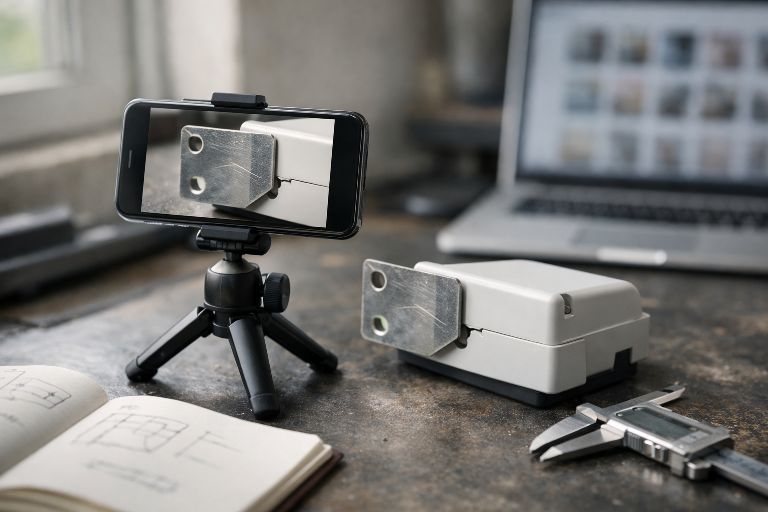
Defect detection with image AI often succeeds or fails before you ever train a model. The biggest lever you control is photo consistency: lighting that doesn’t drift, angles that don’t wander, and framing that keeps the product—not the environment—as the star of the image. This chapter shows how to capture dependable inspection photos with a phone using a fast “micro photo station” you can set up almost anywhere.
Think like a process engineer. Your goal is not to take the prettiest picture; it’s to take the same picture over and over. When the photo process is repeatable, an AI model can learn patterns that correlate with defects rather than “accidents” like a new shadow, a different tabletop, or a slightly different distance. The practical outcome you’re aiming for is a first dataset of 100–300 usable images that are consistent enough to train an “OK vs Defect” classifier later without being misled by noise.
We’ll build a repeatable photo station in about 10 minutes, then create a shot list (angles, distance, and backgrounds). Along the way, you’ll learn how to avoid common failure modes—glare, blur, shadows, and clutter—so defects actually show up in the pixels. Finally, you’ll organize images so labeling and dataset splitting are painless rather than chaotic.
Practice note for Set up a repeatable photo station in 10 minutes: document your objective, define a measurable success check, and run a small experiment before scaling. Capture what changed, why it changed, and what you would test next. This discipline improves reliability and makes your learning transferable to future projects.
Practice note for Create a shot list: angles, distance, and backgrounds: document your objective, define a measurable success check, and run a small experiment before scaling. Capture what changed, why it changed, and what you would test next. This discipline improves reliability and makes your learning transferable to future projects.
Practice note for Avoid common failure modes: glare, blur, shadows, clutter: document your objective, define a measurable success check, and run a small experiment before scaling. Capture what changed, why it changed, and what you would test next. This discipline improves reliability and makes your learning transferable to future projects.
Practice note for Build your first dataset: 100–300 usable images: document your objective, define a measurable success check, and run a small experiment before scaling. Capture what changed, why it changed, and what you would test next. This discipline improves reliability and makes your learning transferable to future projects.
Practice note for Set up a repeatable photo station in 10 minutes: document your objective, define a measurable success check, and run a small experiment before scaling. Capture what changed, why it changed, and what you would test next. This discipline improves reliability and makes your learning transferable to future projects.
Lighting is the most important variable in phone-based inspection photos. Your goal is bright enough to reduce camera noise, soft enough to avoid harsh reflections, and consistent enough that “OK” and “Defect” images differ because of the product, not the light. In practice, you can set up a repeatable photo station in 10 minutes with items you already have: a desk, a plain background (paper or cardboard), and two lamps.
Start with two light sources placed symmetrically at roughly 45° angles to the product—one on the left, one on the right. If you only have one lamp, use a bright window as the second source, but try to shoot at the same time of day to keep it consistent. Make the light soft by diffusing it: tape a sheet of white printer paper in front of the lamp (not touching a hot bulb), or bounce the light off a white wall/foam board. Soft light reduces glare on glossy plastics and metals and makes small surface changes easier to see.
Common mistakes include mixing different color temperatures (yellow lamp plus blue daylight), which shifts colors and can confuse the model. If possible, turn off overhead lights that create extra shadows. Once you find a good setup, don’t keep “improving” it mid-dataset—small lighting changes create two different domains that the model will treat like two different products.
A phone camera can capture excellent inspection data, but only if you control focus, exposure, and motion. Blur is a silent dataset killer: the image may look “fine” on a small screen, but the defect signal disappears when you zoom in or when the model tries to learn edge-level detail.
Stability: Use a simple stand: a small tripod, a phone clamp, or a stack of books with a rubber band. The point is to lock distance and angle so you can repeat shots. If handheld is your only option, brace your elbows on the table and use the 2-second timer to avoid shake. A stable setup also makes it easier to build a shot list because each position is physically repeatable.
Focus: Tap to focus on the actual defect-relevant surface (not the background). Then lock focus if your camera app allows it (AE/AF lock on many phones). If focus drifts between shots, the model learns inconsistent texture. Keep the product at a fixed distance; don’t rely on digital zoom. If you need a closer view, physically move the phone closer or use a lens attachment, but keep that choice consistent across the dataset.
Exposure: Overexposed highlights wash out scratches, dents, and discoloration. Underexposed images bury defects in noise. After tapping to focus, adjust exposure slightly down if shiny areas clip to pure white. Aim for visible detail in both bright and dark areas of the product. Avoid portrait mode and beauty filters; they alter edges and textures in ways that are unhelpful for inspection.
Image AI learns correlations. If your “Defect” photos tend to be shot on a messy workbench and your “OK” photos on a clean table, the model may learn the bench—not the defect. A controlled background and consistent framing reduce these accidental shortcuts.
Choose a background that contrasts with the product but is not visually complex. Matte white or matte gray poster board works for many items; for very light products, use a darker matte background. Avoid glossy surfaces that create reflections of the phone, ceiling lights, or your hands. If the product has holes or edges where the background shows through, use the same background for every shot so the model doesn’t treat background patterns as defect cues.
Framing should be consistent enough that the model sees the same “composition” each time. Decide whether you’re doing full-product classification (whole item in frame) or region-focused classification (only the critical surface). For a beginner “OK vs Defect” classifier, full-product framing often works if defects are visible at that scale. Keep margins consistent: for example, fill 70–80% of the frame with the product and leave a small border of background. Use tape on the table to outline where the product sits and where the phone stand sits.
This is engineering judgment: if defects occur primarily on one face, prioritize that face, but keep at least one “context” shot so the model sees the product identity consistently.
A model can’t learn what the camera doesn’t capture. Defect visibility is about making the defect’s visual signal strong and repeatable. Start by defining what “defect” means operationally: scratches above a certain length, chips on edges, missing components, discoloration, misalignment, contamination, or cracks. Then adjust the capture process so those issues stand out.
Use lighting angle as a tool. For surface defects like scratches or dents, slightly raking light (light coming from a low angle) can cast tiny shadows that reveal texture. For glossy parts that show glare, rotate the product or move lights until specular highlights move away from the critical area. A good rule: if you see a bright white hotspot covering the inspection zone, the camera is blind there.
Plan your shot list around defect-prone zones. Instead of random photos, create a consistent sequence: “Front face (straight-on), Front face (10° tilt), Edge A close-up, Edge B close-up,” etc. The goal is not to maximize variety; it’s to cover critical surfaces with repeatable views. Keep distance consistent for each shot type—mark it physically (tape marks) rather than guessing.
Avoid common failure modes: glare hides texture; blur removes small defects; shadows can look like stains; clutter becomes a cue the model may latch onto. If the defect is extremely small, consider a dedicated close-up shot type rather than expecting the model to infer it from a full-frame image. In early datasets, it’s better to have fewer shot types executed reliably than many shot types captured inconsistently.
Data organization is part of model quality. If you can’t trace an image back to a product instance, a date, and a shot type, you’ll struggle to label consistently and to debug failures later. A simple folder and file naming scheme makes the next chapters (labeling, splitting, training, evaluation) smoother and less error-prone.
Use a top-level project folder, then separate raw captures from curated images. Keep the raw originals untouched so you can reprocess later if needed.
For filenames, pick a pattern that encodes the essentials without being verbose. Example: YYYYMMDD_lineA_product123_shotF_0007.jpg. Include: date (or batch), product/serial (or lot), shot type (F/B/L/R/T/CloseA), and a sequence number. If you have multiple phone stations, add station ID.
Why this matters: when you later discover that a model is failing on “right-side” images or on a specific batch, you can filter instantly. Also, consistent names reduce accidental duplicates and help ensure your train/test split is honest (for example, keeping the same product instance from appearing in both sets). Even if you’re not splitting yet, organize now so you don’t rebuild later under time pressure.
Your first milestone is a small, usable dataset—not a perfect one. For a beginner “OK vs Defect” classifier, target 100–300 usable images captured with the same station, shot list, and camera settings. “Usable” means: in focus, properly exposed, consistent background, and showing the intended shot type. Delete or quarantine borderline images (heavy blur, strong glare on the inspection zone, random backgrounds). A smaller clean dataset beats a larger noisy one at this stage.
A practical starting distribution is roughly balanced: aim for 50–150 OK and 50–150 Defect images. If defects are rare (common in real production), don’t fake balance by photographing the same defect repeatedly from identical angles; instead, collect variety across defect types and locations while keeping the shot process consistent. If you only have a handful of defect items, take multiple shot types per item, but note that this can inflate performance later if similar views end up in both training and testing. Your file naming (product ID) helps prevent that by letting you group images by item.
Build the dataset in passes. Pass 1: capture with the station and shot list. Pass 2: quick review at full zoom to reject blur/glare. Pass 3: ensure each shot type has enough examples (e.g., at least 20 per shot type if you have five angles). Keep a short checklist in your notes: station distance, light positions, background choice, and the exact shot list. The practical outcome is confidence that differences across images are mostly due to the product condition—exactly what an image AI model needs to learn reliably.
1. Why does defect detection with image AI often succeed or fail before you train a model?
2. What is the primary goal when capturing inspection photos for an AI dataset in this chapter?
3. How does a shot list help you build a dependable dataset?
4. Which set of issues does the chapter highlight as common failure modes to avoid so defects show up in the pixels?
5. What practical outcome should you aim for by the end of Chapter 2 before training an OK vs Defect classifier?
You can take excellent product photos and still end up with a disappointing defect detector if your labels are messy. In defect detection, “labeling” means deciding what each image represents in plain business terms: is the product acceptable (OK) or not (Defect)? This chapter turns labeling from a vague chore into a repeatable process you can hand to a teammate and get consistent results.
The key idea is that labels are not just metadata; they are your model’s definition of quality. If your team labels scratches as “Defect” on Monday but “OK” on Tuesday, the model can’t learn a stable rule. If you include borderline images without a plan, the model learns to guess. If you split your data carelessly, you can “accidentally cheat” and report unrealistic accuracy. Good labeling is where engineering judgment shows up: you choose definitions, handle exceptions, and set up checks so the dataset stays trustworthy.
In this chapter you’ll write a simple labeling rulebook, label OK vs Defect (including “maybe” cases), balance the dataset so learning is fair, and split images into train/validation/test without leakage. You’ll also do a quick quality pass to catch common mistakes before you spend time training a model on bad data.
Practice note for Write a labeling rulebook in plain language: document your objective, define a measurable success check, and run a small experiment before scaling. Capture what changed, why it changed, and what you would test next. This discipline improves reliability and makes your learning transferable to future projects.
Practice note for Label images as OK vs Defect (and handle “maybe” cases): document your objective, define a measurable success check, and run a small experiment before scaling. Capture what changed, why it changed, and what you would test next. This discipline improves reliability and makes your learning transferable to future projects.
Practice note for Balance the dataset so the model learns fairly: document your objective, define a measurable success check, and run a small experiment before scaling. Capture what changed, why it changed, and what you would test next. This discipline improves reliability and makes your learning transferable to future projects.
Practice note for Split data properly: train, validation, and test: document your objective, define a measurable success check, and run a small experiment before scaling. Capture what changed, why it changed, and what you would test next. This discipline improves reliability and makes your learning transferable to future projects.
Practice note for Write a labeling rulebook in plain language: document your objective, define a measurable success check, and run a small experiment before scaling. Capture what changed, why it changed, and what you would test next. This discipline improves reliability and makes your learning transferable to future projects.
In supervised image AI, the model learns by matching pixels to labels. That means labels are the “answer key,” and every wrong or inconsistent label teaches the model the wrong lesson. For defect detection, this effect is amplified because defects are often subtle: tiny dents, hairline cracks, small stains, or misalignments. The model can’t read your mind—it only sees patterns correlated with the labels you provide.
Before labeling anything, define the task precisely: are you detecting cosmetic defects, functional defects, or both? Are you labeling based on what the customer would accept, what QC would accept, or what triggers rework? Your labels should mirror the decision you want the model to automate. If the production rule is “reject if scratch length > 3 mm,” then the dataset should reflect that rule, not each labeler’s personal tolerance.
Use a simple OK vs Defect scheme at the start. It reduces complexity and makes it easier to debug. Multi-class labeling (scratch vs dent vs stain) can come later, after you have a reliable pipeline. Also decide what your unit of labeling is: one whole photo equals one label. If a photo shows multiple items, either crop to one item per image or treat it as “Defect” if any item is defective—write that down.
Think of labeling as product specification work. Once the labels are stable, training becomes a technical step. Without stable labels, training is just repeatedly fitting noise.
A defect checklist is a beginner-friendly way to turn quality standards into consistent labels. It should be short, concrete, and written in plain language. The checklist is also the heart of your labeling rulebook: it tells labelers exactly what counts as Defect and what counts as OK.
Start by listing 5–10 defect types you actually see in the line. For each one, write (1) what it looks like, (2) where it typically appears, and (3) the acceptance threshold. Avoid vague terms like “minor” or “significant” unless you define them. If you can measure it (length, area, color shift, missing component), define a simple threshold.
Examples make the checklist usable. Create a small “golden set” folder of reference images: 10–20 clear OK examples and 10–20 clear Defect examples. If possible, include one example per defect type and one example of a common false alarm (e.g., reflections that look like scratches). When a new labeler joins, have them label the golden set first; if they disagree, update the rulebook or clarify the examples.
Engineering judgment: choose thresholds that match business cost. If missing a defect is expensive, you may label more borderline items as Defect so the model learns a stricter boundary. If false alarms are expensive (stopping a line), you may be more conservative. The important point is consistency: pick a policy, document it, and label accordingly.
Real datasets contain “maybe” images: borderline scratches, ambiguous shadows, or photos that are slightly out of focus. If you force every image into OK or Defect without a plan, you inject noise. If you delete all hard cases, the model will look great in testing but fail in production. The solution is to define how you handle uncertainty.
Use a three-bucket workflow during labeling, even if your final model is binary:
“Review” is not a permanent label; it is a queue. Decide who resolves it (a senior inspector, team lead, or consensus meeting) and how. A practical approach is double-labeling: two people label the same subset (say 10–20%) and you measure agreement. Where they disagree, you don’t just pick a winner—you learn what rule is missing. Often the fix is adding a specific example or clarifying a threshold.
Borderline cases can be handled in a few ways:
Common mistake: silently labeling uncertain images as OK because it “feels safer.” This teaches the model that true defects are OK, increasing misses. If you must bias one direction, do it deliberately and document it (for example: “When unsure, label as Defect to reduce customer escapes”).
Most production lines produce mostly OK products. That’s good for the business but dangerous for model learning. If 95% of your images are OK, a lazy model can predict “OK” for every photo and still achieve 95% accuracy. This is why class balance matters: the model must see enough Defect examples to learn what defects look like, not just what “normal” looks like.
Balancing does not mean forcing a 50/50 dataset in every case, but you do need sufficient defect diversity. A practical starting point for a basic OK vs Defect classifier is to aim for at least 20–30% Defect images in the training set, as long as they represent the real defect types you care about. If defects are rare, you can oversample by collecting more defect examples intentionally (e.g., from rework bins, historical rejects, controlled creation of known defects if allowed).
Engineering judgment: you can intentionally skew training data toward Defects to teach sensitivity, then later adjust decision thresholds to reduce false alarms. But if you hide the true production ratio entirely, you may misinterpret metrics. Keep a note of the real-world defect rate and compare model behavior under both balanced training and realistic testing.
Common mistake: balancing by taking all OK images from one day and all Defect images from another. That introduces hidden signals (shift changes, camera position, lighting) that the model may use instead of the defect itself. Balance should be done while keeping capture conditions comparable across classes.
After labeling, the next critical step is splitting data into train, validation, and test. The goal is to measure performance on images the model truly has not seen. “Leakage” happens when the model indirectly sees the test data during training—often by including near-duplicate images across splits.
Use this simple split purpose statement:
A practical default split is 70/15/15 or 80/10/10, but the exact ratios matter less than preventing leakage. In inspection, leakage commonly comes from burst photos: you take 5 shots of the same product seconds apart. If some go to train and others to test, the model “recognizes” that product rather than learning defect features. Fix this by splitting by group, not by image. Group by product serial number, batch, time window, or capture session folder, and ensure the entire group goes into only one split.
Also split with future deployment in mind. If you expect lighting or background changes over time, consider a time-based split: earlier dates for training, later dates for testing. This is tougher but often closer to reality.
Common mistakes:
Practical outcome: a clean split lets your accuracy, misses, and false alarms reflect how the model will behave on new photos—so later chapters’ training and evaluation steps aren’t misleading.
Before training, do a short labeling QA pass. This takes minutes to hours, not days, and it can save weeks of confusion. The goal is to catch systematic issues: swapped labels, inconsistent interpretation, and hidden shortcuts the model could learn (background cues, stickers, or hands in frame).
Run this practical checklist:
Then do one “rulebook test”: hand 20 unlabeled images to a second person plus the rulebook and checklist. Compare labels. If disagreements cluster around one defect type, your definition is unclear. Update the rulebook and relabel the affected subset now, before training locks in the confusion.
Common mistake: assuming the model will “average out” labeling noise. In practice, labeling noise often becomes performance noise: random misses, unpredictable false alarms, and a model that behaves differently across shifts. A quick QA pass turns labeling into a controlled process—and makes the next chapter’s model training much more straightforward.
1. Why does the chapter emphasize writing a labeling rulebook in plain language?
2. What is the main risk if your team labels the same type of flaw (e.g., scratches) as “Defect” one day and “OK” another day?
3. How should “maybe” or borderline images be handled according to the chapter’s approach?
4. What is the purpose of balancing the dataset when labeling OK vs Defect images?
5. Why does the chapter warn about splitting data carelessly into train/validation/test sets?
In the previous chapters you built the foundation: consistent photos, a defect checklist, and labels that a computer can learn from. Now you’ll turn that labeled folder of images into a working “OK vs Defect” classifier. The goal of this chapter is not to chase perfection—it’s to produce a trustworthy first model, understand what it’s doing, and set up habits that prevent misleading results later.
We’ll use a beginner-friendly training tool (for example: a no-code/low-code image classifier in a desktop app, a cloud AutoML interface, or a simple notebook template). Regardless of the tool, the workflow is the same: load your dataset, choose basic settings, train a baseline model, test it with new photos taken today, and then save/version the model like a real project.
As you work through the steps, keep one practical idea in mind: your model is only as reliable as the “story” your data tells. If your Defect photos are all darker than your OK photos, your model may learn lighting instead of defects. If your training and test photos are near-duplicates, accuracy can look great while real-world performance is poor. The best beginners’ advantage is discipline: consistent capture, clean splits, and careful notes.
Let’s train your first model.
Practice note for Use a beginner-friendly training tool and load your dataset: document your objective, define a measurable success check, and run a small experiment before scaling. Capture what changed, why it changed, and what you would test next. This discipline improves reliability and makes your learning transferable to future projects.
Practice note for Train a baseline model and understand what happened: document your objective, define a measurable success check, and run a small experiment before scaling. Capture what changed, why it changed, and what you would test next. This discipline improves reliability and makes your learning transferable to future projects.
Practice note for Test with new photos taken today: document your objective, define a measurable success check, and run a small experiment before scaling. Capture what changed, why it changed, and what you would test next. This discipline improves reliability and makes your learning transferable to future projects.
Practice note for Save and version your model like a real project: document your objective, define a measurable success check, and run a small experiment before scaling. Capture what changed, why it changed, and what you would test next. This discipline improves reliability and makes your learning transferable to future projects.
Practice note for Use a beginner-friendly training tool and load your dataset: document your objective, define a measurable success check, and run a small experiment before scaling. Capture what changed, why it changed, and what you would test next. This discipline improves reliability and makes your learning transferable to future projects.
Training is the process of showing your computer many examples of each label (here: OK and Defect) so it can learn visual patterns that tend to go with each label. Think of it like training a new inspector: at first they guess; after seeing many products, they start noticing repeatable cues—scratches, chips, dents, discoloration, missing parts, or misalignment. A model does the same, but it learns “cues” as combinations of pixels, edges, textures, and shapes.
Beginner-friendly tools hide the math, but you still need to control the inputs. When you “load your dataset,” the tool typically asks for folders or a CSV/manifest that maps each image to a label. Your responsibility is to ensure: (1) labels are correct, (2) images match the same inspection view(s), and (3) the dataset split is honest (no leaking near-identical photos into both training and test).
Common mistake: treating training as “press a button.” If the tool gives high accuracy quickly, don’t celebrate yet. First ask: are OK and Defect photos captured under the same lighting and background? Are there any “shortcut signals” (a sticky note, a different table, a different camera) that correlate with the label? A surprising amount of defect-detection failure comes from the model learning the wrong thing very confidently.
Start with the simplest useful question: “Should this product be flagged for review?” That is an OK vs Defect classifier. It’s a baseline because it sets a clear reference point for future improvements (like multi-class defect types or defect localization). Baselines are not “low quality”—they are how professional projects reduce risk and discover data problems early.
In your training tool, create two classes: OK and Defect. Load images from your labeled folders. If your dataset is imbalanced (for example, 900 OK and 80 Defect), don’t panic, but do acknowledge it: the model may learn to say “OK” too often and still look accurate. If possible, collect more Defect examples or use careful evaluation metrics (misses vs false alarms) rather than accuracy alone.
Engineering judgment: define what you’re optimizing for. In many inspection lines, a missed defect (false negative) is worse than a false alarm, because a missed defect ships. That means your baseline might accept more false alarms if it dramatically reduces misses. Write this down now; it will guide threshold choices and future data collection.
Most training tools ask for an image size (resolution) and offer augmentation. These two settings can make or break a beginner project because they determine what details the model can “see” and how robust it becomes to normal variation.
Image size: If defects are tiny (hairline cracks, small pits), resizing images too small can erase the signal. As a practical starting point, choose a medium resolution your tool supports (often 224×224, 320×320, or 512×512). If your defects are subtle, prefer the higher option—while accepting longer training time. If defects are large (missing component, big dent), lower sizes may work fine. The key is to match resolution to defect scale.
Augmentation: Augmentation creates modified copies of training images (small rotations, brightness shifts, slight zoom, minor crops) to help the model handle real-world variation. Use it to simulate the variation you expect on the line, not to create chaos.
Practical workflow: train once with conservative augmentation. If the model fails on today’s new photos (Section 4.5), increase augmentation gradually rather than changing everything at once. If your tool supports it, also consider “center crop” vs “fit” behavior; inconsistent cropping can hide the defect area. Your capture setup from earlier chapters (consistent distance and framing) reduces how much you need augmentation at all.
When you press “Train,” the tool runs a training loop in repeated passes through the training images. Each pass is an epoch. After each epoch, the tool reports performance on the validation set. You don’t need the math, but you do need to read the story those curves tell.
Epochs: More epochs can improve learning—up to a point. Early on, both training and validation performance often improve. If training keeps improving but validation gets worse, you’re likely overfitting (memorizing the training set instead of learning general patterns).
Learning rate and presets: Many beginner tools offer presets like “fast,” “balanced,” or “accurate,” which implicitly adjust learning rate and training duration. Start with the default or “balanced.” If results are unstable (metrics jump wildly), slower settings can help. If training is extremely slow, reduce image size slightly or limit epochs—but don’t shrink so much you lose defect detail.
Baseline expectation: your first model may not be production-ready. That’s normal. What matters is learning which errors it makes. Does it miss defects under glare? Does it false-alarm on harmless reflections? Those observations translate directly into better photo capture rules and targeted data collection.
Testing on unseen images is where you find out if your model is useful. Do two kinds of tests: (1) evaluate on your held-out test set, and (2) run predictions on new photos taken today under realistic conditions. The second test is the closest to real deployment and often reveals issues that your curated dataset hides.
Most tools output a predicted label plus a confidence score (for example, “Defect: 0.78”). Treat confidence as a ranking signal, not truth. A practical approach is to set a review threshold: above the threshold, the item is flagged for human review; below it, it passes. If your project prioritizes safety, choose a lower threshold to reduce misses, accepting more false alarms.
Practical procedure for today’s photos: take 20–50 images following your capture standard (same lighting, angle, distance). Include a few intentionally difficult cases: minor glare, slight rotation, borderline defects. Label them after capture using your checklist, then compare to the model’s predictions. Write down patterns: “misses occur when the defect is near the edge,” or “false alarms occur on a certain shiny region.” These notes drive your next data collection and potential cropping/ROI strategies in later chapters.
Once you have a baseline model, start treating it like a real project asset. “Model versioning” means you can answer two questions later: Which model made this decision? and What data/settings produced it? Without this, teams get stuck in confusion—accuracy changes, nobody remembers why, and trust in the system drops.
Create a simple version naming scheme and a small “model card” text file saved alongside the exported model. You don’t need heavy tools to begin; a folder structure and consistent notes are enough.
defect_ok_v0.1, v0.2, etc.Also save example misclassifications (a few images the model got wrong) in a “known issues” folder. Those images become your regression test later: when you retrain with more data, you can quickly check whether the new model fixes old mistakes without introducing new ones.
Practical outcome: by the end of this chapter you should have (1) a trained baseline classifier, (2) evidence from new photos taken today, and (3) a versioned model artifact with notes. That combination turns “I trained something” into a repeatable inspection workflow you can improve safely.
1. What is the main goal of Chapter 4 when training your first “OK vs Defect” model?
2. Which workflow best matches the chapter’s recommended process regardless of the training tool you choose?
3. Why can a model appear accurate but perform poorly in the real world, according to the chapter?
4. What risk is illustrated by the example where Defect photos are darker than OK photos?
5. Which set of metrics does the chapter highlight as useful for understanding your baseline classifier?
You can’t improve what you don’t measure. In defect detection, “measure” does not mean chasing a single number until it looks good. It means translating model behavior into shop-floor consequences: How many bad parts slip through? How many good parts get stopped? How much rework time do false alarms create? This chapter gives you a practical, data-first routine for evaluating an “OK vs Defect” photo model and then fixing the real causes of errors—usually photo consistency, label noise, and missing coverage.
A common beginner mistake is to treat model training like cooking: change a hyperparameter, stir, and hope it tastes better. In practice, most failures come from the dataset. If the model can’t see a defect clearly (lighting/angle/distance), or if “Defect” labels mix several different failure modes without enough examples of each, no amount of tuning will rescue it. Your job is to build a feedback loop: evaluate → inspect errors → identify patterns → collect the missing examples → relabel/clean → retrain.
By the end of this chapter you will be able to read a confusion matrix in plain language, set a decision threshold to control false alarms vs misses, and run an error-review workflow that converts “the model is wrong” into specific actions: “we need 30 more examples of scratches under warm light,” or “these labels are inconsistent,” or “our camera distance varies too much.”
Keep your evaluation set separate. If you change your data or process, re-evaluate on the same held-out test set where possible, or keep a “golden” set that represents real production conditions. Otherwise you’ll reward yourself for overfitting and believe the system is improving when it’s only memorizing.
Practice note for Read a confusion matrix in plain language: document your objective, define a measurable success check, and run a small experiment before scaling. Capture what changed, why it changed, and what you would test next. This discipline improves reliability and makes your learning transferable to future projects.
Practice note for Set a decision threshold to control false alarms vs misses: document your objective, define a measurable success check, and run a small experiment before scaling. Capture what changed, why it changed, and what you would test next. This discipline improves reliability and makes your learning transferable to future projects.
Practice note for Find failure patterns and collect “missing” examples: document your objective, define a measurable success check, and run a small experiment before scaling. Capture what changed, why it changed, and what you would test next. This discipline improves reliability and makes your learning transferable to future projects.
Practice note for Improve results with better photos, labels, and coverage: document your objective, define a measurable success check, and run a small experiment before scaling. Capture what changed, why it changed, and what you would test next. This discipline improves reliability and makes your learning transferable to future projects.
Practice note for Read a confusion matrix in plain language: document your objective, define a measurable success check, and run a small experiment before scaling. Capture what changed, why it changed, and what you would test next. This discipline improves reliability and makes your learning transferable to future projects.
Practice note for Set a decision threshold to control false alarms vs misses: document your objective, define a measurable success check, and run a small experiment before scaling. Capture what changed, why it changed, and what you would test next. This discipline improves reliability and makes your learning transferable to future projects.
Practice note for Find failure patterns and collect “missing” examples: document your objective, define a measurable success check, and run a small experiment before scaling. Capture what changed, why it changed, and what you would test next. This discipline improves reliability and makes your learning transferable to future projects.
Start with three metrics you can explain to anyone on the line: accuracy, precision, and recall. You do not need a long list of statistics to make good decisions, but you do need to understand what each one hides.
Accuracy is “what percent did we get right overall.” If you inspected 1,000 photos and the model was correct on 950, accuracy is 95%. The trap: accuracy can look great when defects are rare. If only 2% of items are defective, a model that predicts “OK” for everything is 98% accurate—and completely useless.
Recall (for “Defect”) answers: “Of the truly defective items, how many did we catch?” This is the metric tied to misses (defects slipping through). If you had 100 defective parts and caught 90, defect recall is 90% and misses are 10%. When safety, warranty returns, or customer trust are on the line, recall often matters most.
Precision (for “Defect”) answers: “When we flag a defect, how often are we right?” This is tied to false alarms (good parts stopped). If the model flags 200 parts as defective but only 100 are truly defective, precision is 50% and you’ve created a lot of unnecessary review/rework.
Engineering judgment is choosing the right balance. A medical device housing might demand extremely high recall (almost no misses), accepting some false alarms. A high-volume, low-risk product might prioritize precision so operators are not overwhelmed. Write your target in plain language: “We can tolerate 1 miss per 5,000 parts, but false alarms must be under 3% so the recheck station doesn’t back up.” Then pick metrics that match that statement.
A confusion matrix turns abstract metrics into counts you can reason about. For a two-class “OK vs Defect” model, it’s a 2×2 table of what was predicted versus what was true. Read it like a production report, not like a math exercise.
Use the four outcomes:
Now translate into plain language questions: “How many bad parts did we miss?” (FN) and “How many good parts did we unnecessarily stop?” (FP). Those two numbers often matter more than the totals.
Common mistake: evaluating on a test set that doesn’t reflect real production variety. If your test set contains mostly clean, well-lit photos, the confusion matrix will look great, but the first week on the line will expose failures under glare, shadows, motion blur, or new defect types. Your confusion matrix should come from photos captured using the same phone setup, lighting, distance, and angle constraints you defined earlier in the course.
When the matrix looks bad, don’t immediately blame the model. Ask: “Is the label correct?” “Is the photo usable?” “Is this defect even visible?” If a defect can’t be seen at your standard capture distance, the right fix may be a photo process change (closer shot or raking light), not more training epochs.
Most classifiers don’t just output “OK” or “Defect.” They output a probability-like score (for example, 0.0 to 1.0) representing how confident the model is that the photo shows a defect. The decision threshold is the cutoff you choose to convert that score into a yes/no decision.
If your threshold is 0.50, then scores ≥ 0.50 become “Defect.” If you raise the threshold to 0.80, the model becomes more conservative: it will flag fewer photos as defects. That usually reduces false alarms (FP goes down) but increases misses (FN goes up). If you lower the threshold to 0.20, the model becomes stricter: it flags more photos as defects, usually catching more true defects (FN down) but causing more false alarms (FP up).
Pick a threshold based on your process capacity and risk, not based on what looks nice in a chart. A practical workflow is to test several thresholds on your validation set and write down the resulting confusion matrix counts. Then decide: Can your team review 50 flagged items per hour? What’s the cost of one missed defect compared to one extra review?
Two common deployment patterns:
Do not change the threshold using your final test set. Treat the threshold like a setting you tune on a validation set, then lock it before reporting final performance, so your results stay honest.
Once you have a confusion matrix, your next job is to inspect the photos behind the errors. This is where improvement actually happens. Create an “error review” folder or spreadsheet with four tabs: FP, FN, TP, TN. Prioritize FN first (missed defects), then FP (false alarms), because those are the operational pain points.
A simple, repeatable workflow:
Common mistake: treating every error as unique. Your goal is to find repeatable failure modes. For example, if the model misses scratches only when the product is rotated 30 degrees, you’ve discovered a coverage gap: your training data doesn’t include that rotation, or your photo checklist didn’t enforce orientation.
Also review a sample of “correct” predictions. Sometimes the model is “right for the wrong reason,” such as learning the background color or a sticker that correlates with defects. If TN photos always come from one workstation and TP from another, the model may be detecting workstation differences, not defects.
Most improvement in beginner defect systems comes from data quality and coverage, not from a fancier model. Use your error review categories to drive specific data fixes.
Add hard cases (coverage fixes). Collect more examples that represent the failure patterns: glare, shadows, warm/cool lighting, slight angle shifts, different phone operators, different batches of material, and defects at the smallest size you care about. If you only add “easy” defects (large cracks in perfect light), your recall on subtle defects won’t move. A good rule is to add data where the model is uncertain (scores near your threshold) and where it is confidently wrong (high-score false alarms or low-score missed defects).
Improve photo consistency (signal fixes). If many errors involve blur or distance changes, fix the capture process: mark a fixed shooting distance, use a simple jig, add diffuse lighting, or lock phone exposure. Better photos often outperform adding hundreds of noisy images.
Remove label noise (truth fixes). Inconsistent labels cap performance. If one person labels minor scuffs as “OK” and another labels them “Defect,” the model learns confusion. Revisit your defect checklist and define boundaries with example photos: “Scratch longer than 5 mm is Defect,” or “Cosmetic mark allowed in Zone C.” Then relabel a small set of disagreements and measure if metrics improve.
Balance intelligently. You don’t always need equal counts of OK and Defect, but you do need enough defect examples per defect type. If “Defect” includes cracks, dents, and contamination, ensure each appears frequently enough. If one type has only 10 examples, the model will likely miss it—so treat that as a data collection requirement, not a surprise.
Teams often get stuck in endless iteration because they never define success. “Higher accuracy” is not a stopping rule. Define “good enough” based on the cost of mistakes, the stability of results, and the effort required to improve further.
Start with an operational target stated in counts over time, not just percentages: “On a representative test set of 2,000 items with 100 defects, we need at most 2 missed defects (FN ≤ 2) and no more than 60 false alarms (FP ≤ 60).” This forces you to think in realistic volumes. If defects are rare, increase test set size; otherwise your metrics will swing wildly from week to week.
Next, check stability. Evaluate on different days, operators, and batches. If performance collapses when lighting changes slightly, you are not ready to deploy a hard gate. You might still be ready for an “assist” mode where a human makes the final call and you keep collecting data.
Finally, consider the data-first ROI. If your remaining errors are mostly “defect not visible in the photo,” the best next step is not more training—it is changing the capture method (closer image, different angle, better light) or adding a second photo. Stop iterating on the model when the limiting factor is physics or process, not learning.
A practical stopping point for early deployments is: consistent capture process in place, a locked threshold that matches review capacity, an error review routine scheduled (weekly or per batch), and a plan for handling unknowns (new defect types routed to human review and added to the dataset). That turns your model from a one-time project into a controlled inspection system that improves with real production data.
1. In this chapter, what does it mean to “measure” a defect-detection model well?
2. What is a key purpose of using a confusion matrix for an OK vs Defect model?
3. How does changing the decision threshold affect inspection behavior?
4. According to the chapter, why do many real-world failures persist even after hyperparameter tuning?
5. Why should you keep an evaluation set separate (or maintain a “golden” set) while iterating?
Training a classifier that can label photos as “OK” or “Defect” is a major milestone—but it is not yet an inspection system. Real inspections need a repeatable workflow a teammate can follow, clear decisions that connect predictions to actions, and enough traceability to explain what happened later (especially when customers or regulators ask). This chapter turns your model into a simple end-to-end photo inspection flow: capture, run, decide, log, and improve.
Think like an engineer responsible for operations. Your goal is not to maximize a metric on a test set; your goal is to reduce escapes (defects incorrectly passed) and reduce waste (good parts unnecessarily blocked), while keeping inspection fast and consistent. That requires practical judgment: setting thresholds, defining retake rules, choosing where the model runs (phone, laptop, or cloud), and designing a reporting log that is lightweight but useful.
We will build a “first workable” workflow. It should be simple enough for a new operator to learn in one session, but structured enough that you can improve it over time. By the end, you will have a step-by-step inspection flow, a basic user experience, operational checks for photo quality, a logging plan for auditability, and a roadmap for upgrading from “defect/no defect” to locating the defect.
Practice note for Design a step-by-step inspection flow a teammate can follow: document your objective, define a measurable success check, and run a small experiment before scaling. Capture what changed, why it changed, and what you would test next. This discipline improves reliability and makes your learning transferable to future projects.
Practice note for Decide where the model runs: phone, laptop, or cloud: document your objective, define a measurable success check, and run a small experiment before scaling. Capture what changed, why it changed, and what you would test next. This discipline improves reliability and makes your learning transferable to future projects.
Practice note for Create a basic reporting log for traceability: document your objective, define a measurable success check, and run a small experiment before scaling. Capture what changed, why it changed, and what you would test next. This discipline improves reliability and makes your learning transferable to future projects.
Practice note for Plan next upgrades: locating defects and expanding products: document your objective, define a measurable success check, and run a small experiment before scaling. Capture what changed, why it changed, and what you would test next. This discipline improves reliability and makes your learning transferable to future projects.
Practice note for Design a step-by-step inspection flow a teammate can follow: document your objective, define a measurable success check, and run a small experiment before scaling. Capture what changed, why it changed, and what you would test next. This discipline improves reliability and makes your learning transferable to future projects.
A model output is not an action. Most image classifiers produce a probability or confidence score (for example, “Defect: 0.72”). If you treat that as a simple yes/no without rules, two operators will interpret it differently, and your results will drift. The workflow needs explicit decision bands that convert predictions into actions a teammate can follow every time.
A practical three-outcome policy works well for beginners:
Example thresholds (you will tune them): if P(Defect) ≥ 0.85 → Fail; if P(Defect) ≤ 0.15 → Pass; otherwise → Recheck. Why not 0.50? Because inspection costs are asymmetric: a missed defect (false negative) is usually more expensive than a false alarm. By widening the Recheck band you reduce escapes at the cost of more retakes or manual checks.
Common mistake: choosing thresholds based only on accuracy. Accuracy can look great even if the model still misses the rare, costly defects. Instead, set thresholds using your test set confusion matrix and focus on misses (false negatives) vs false alarms (false positives). Then align the band widths with your process capacity: how many items per hour can you manually recheck?
Document the rule as a short “inspection decision table” and post it at the station. A workflow you can explain beats a clever workflow no one follows.
Your first inspection tool does not need a complex app. It needs a predictable loop: capture/upload → model result → operator next step → log. If any step is confusing, operators will work around it (and your data quality will collapse). Design the smallest user experience that still enforces consistency.
A practical “version 1” UX can be:
Where does the model run? Choose based on speed, privacy, and connectivity:
Engineering judgment: for a pilot, a laptop-based tool is often the sweet spot—fast enough, controlled hardware, and easy to iterate. If operators must walk away from the part to use the laptop, though, the workflow may fail. Always optimize for physical reality: where the part sits, how hands move, and how quickly decisions must be made.
Common mistake: showing only “OK/Defect” with no next-step instruction. The UI must close the loop, otherwise results become “interesting information” rather than an inspection action.
In production, most “model failures” are actually photo failures. Your model learned from a particular photo style: lighting, distance, background, and angle. If daily photos drift away from that style, confidence drops and errors rise. The fix is not immediately retraining—it is operational control: simple capture rules and explicit retake criteria.
Start with three lighting rules that are easy to teach:
Add framing and distance rules. For example: “Part centered, fills 60–80% of the frame; camera 25 cm from the surface; same orientation marker at top-left.” If you can, use a simple jig: taped outline on the table, phone stand, and a background mat. Jigs feel “low tech,” but they often deliver the highest ROI in defect detection because they reduce variance.
Define retake criteria as a checklist the operator can apply in seconds:
Common mistake: relying on the model to handle poor images. A classifier trained on clean images may confidently misclassify a blurry defect as “OK.” Treat image quality as a first-class inspection gate: the operator should be allowed (and encouraged) to recheck by retaking the photo before accepting a Pass/Fail decision.
Practical outcome: fewer “mystery” false alarms and fewer missed defects, without changing the model at all.
If you cannot explain how an item was inspected, you do not have a dependable inspection process. Logging provides traceability: what was inspected, when, with what result, and what action was taken. It also creates the dataset you will need for improvements and for investigating escapes.
Keep the log lightweight so it actually gets used. A basic reporting log can be a spreadsheet, database table, or even a CSV export from your inspection tool. Minimum recommended fields:
Two practical tips make logs far more valuable. First, separate model prediction from final decision. If an operator overrides a result, capture that override—this is gold for retraining and for understanding failure modes. Second, capture the reason for Recheck/Fail using a small controlled list (e.g., “glare,” “blur,” “scratch,” “dent,” “unknown”). Avoid free-text fields as the primary signal; they become inconsistent quickly.
Common mistake: saving images without a stable naming convention. Use a pattern that embeds time and batch, such as SKU123_LOT45_2026-03-27T101530Z_camA.jpg. When something goes wrong, the ability to locate the exact photo in seconds is the difference between a calm investigation and a chaotic one.
A simple “OK vs Defect” model is powerful, but it is not magic. Real-world inspection systems degrade over time due to drift: changes in the product, environment, or capture device that shift the image distribution away from what the model learned.
Plan for these common sources of drift:
Mitigations should be operational first, then model-based. Operationally: lock down the photo station (same light, same stand), and include quick daily checks (take one known-good reference photo and confirm the model outputs Pass with high confidence). Model-based: track monthly metrics using your log (false alarms, misses found downstream, and recheck rate). A rising recheck rate is often the earliest warning sign of drift.
Common mistake: retraining on whatever images are easiest to collect. If you only retrain on “easy” OK images, the model may appear stable but still miss rare defects. When a new defect appears, capture and label it deliberately, and keep it as a “challenge set” you evaluate every release.
Practical outcome: you treat the model as a maintained component of the workflow, not a one-time project.
Once your classification workflow is stable, the next limitation becomes obvious: “Defect” does not tell you where the issue is. Operators and repair technicians often need localization to work faster, and engineers need it to understand root cause. Upgrading from classification to location is the natural next step.
There are two practical upgrade paths:
Expanding products is another common next step. If you add more SKUs or variants, decide whether to train one model per product family or a single multi-class model. Start by adding products that look similar and share defect modes; mixing visually unrelated products too early can increase confusion and reduce reliability.
Engineering judgment: do not rush into detection if your capture process is still inconsistent. Localization models are usually more sensitive to camera angle, scale, and lighting. First stabilize the workflow (Sections 6.1–6.4), then invest in richer labels.
A practical plan is incremental: keep your current classifier as a gate (fast Pass vs not-Pass), send Recheck/Fail cases to a localization model or a manual step, and use the logged images to steadily build the labeled dataset needed for full defect location.
1. Why does a photo classifier that outputs only “OK” or “Defect” still not qualify as a complete inspection system?
2. What is the primary operational goal of the workflow described in this chapter?
3. Which set of steps best matches the end-to-end inspection flow the chapter aims to build?
4. What is the purpose of setting thresholds and defining retake rules in the inspection workflow?
5. Why does the chapter recommend creating a basic reporting log for traceability?
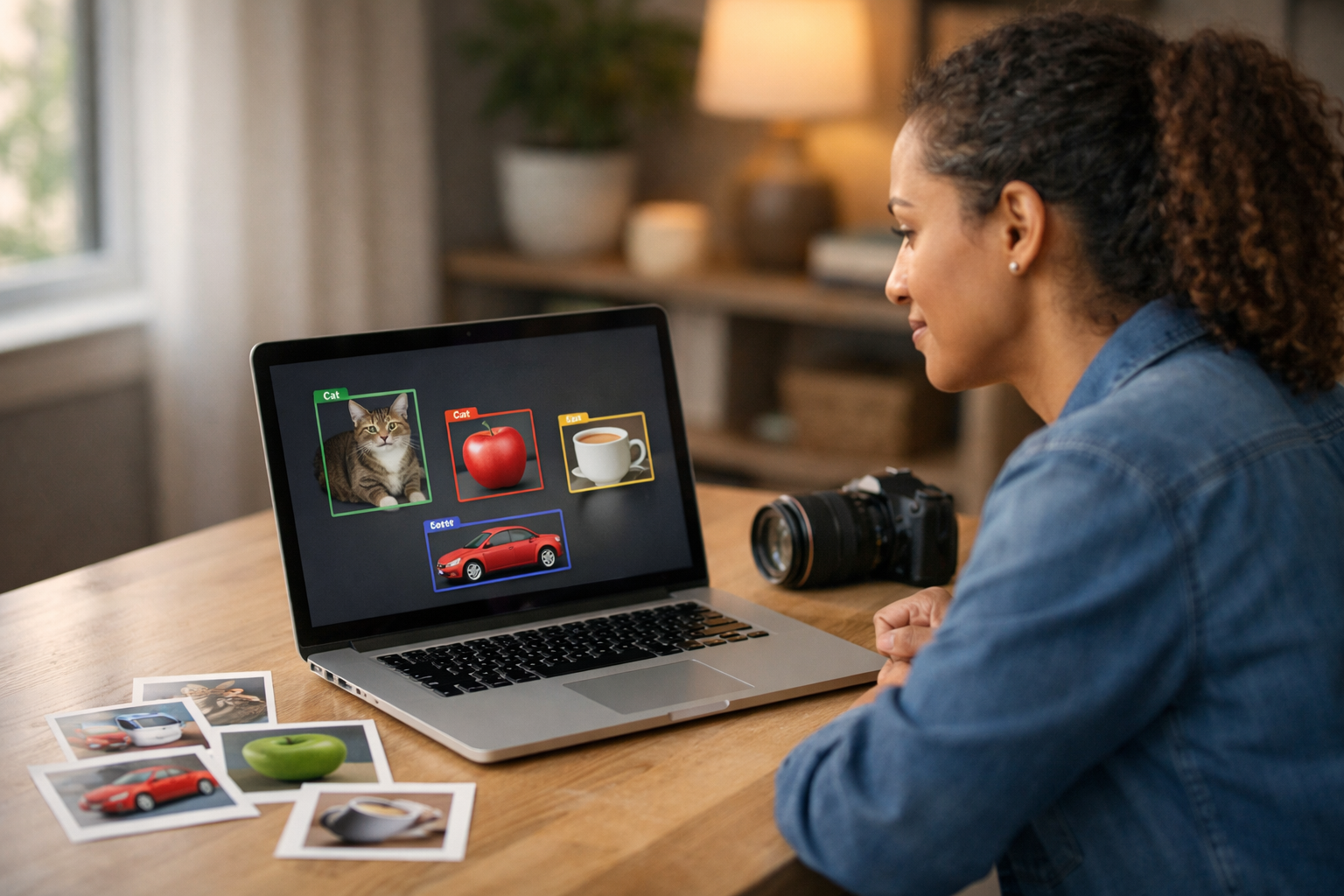
- Learning Evolved.
- Intelligence Amplified.